Biggest takeaways from our RL tutorial: Long-term rewards, offline RL, and more

I am typing this shortly after the Production RL Summit, a virtual event for reinforcement learning (RL) practitioners hosted by Anyscale. The event concluded with a hands-on tutorial on Ray RLlib for building recommender systems, led by the lead maintainer of RLlib, Sven Mika. As someone who helped create the tutorial, it was rewarding to see an engaged and enthusiastic audience of 170 students, actively writing code and using Ray RLlib! In this blog post, I’ll share a quick summary of the tutorial, along with a few of my big takeaways.

LinkGetting started

The tutorial started off with an introduction to RL and how RL can be applied to recommender systems, or RecSys. Basically, RL requires 1) an environment outputting observations and a reward signal, and 2) an algorithm. Then 3) an agent explores the environment (or simulation) to find which actions give the best sum of (individual, per-timestep) rewards. This can be applied to the specific user-interactions of RecSys when a user is exploring, searching, and clicking. In this way, the user as well as the interface (for example, a browser) is part of the simulation (or RL environment), and the goal of the RecSys is to serve up the best click-options to the user at exactly the right time to maximize the user’s satisfaction (reward). “K-Slate” means there are K things to be recommended at once. You have probably seen this while browsing — the sliding window of recommended videos to watch, songs to play, images requesting your reaction, products to buy, or meals to order.

Each student had their own, provisioned Python 3.9 cluster on Anyscale (backend AWS EC2) with Ray, RLlib, OpenAI gym, Google’s RecSim environment, JAX, and PyTorch pre-installed.  Also pre-installed was the Jupyter tutorial notebook.

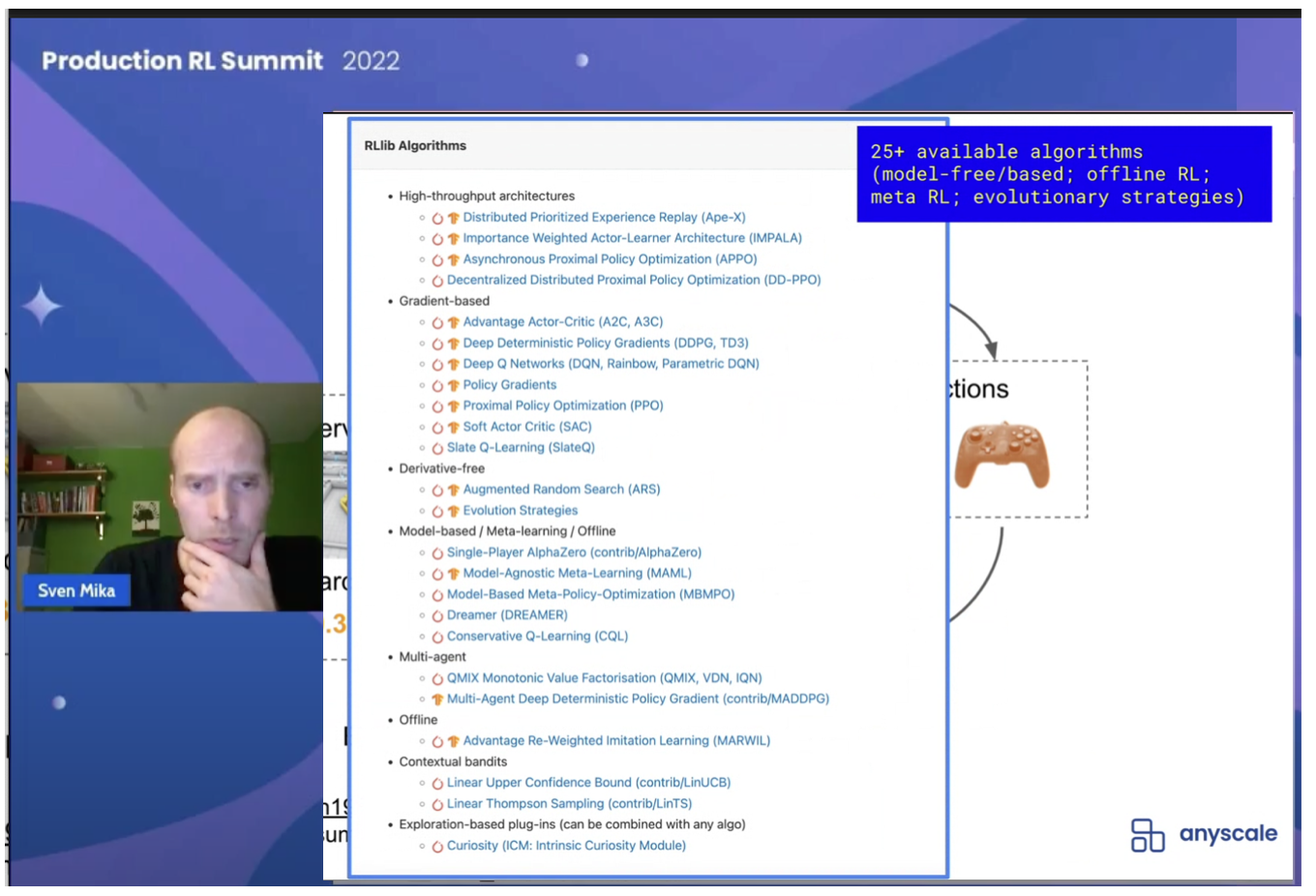
Open-source RLlib contains 25+ available algorithms, all converted to both TF2 and PyTorch, easily runnable as either single- or multi-agents, covering different sub-categories of RL: model-based, model-free, offline RL. Because it runs on Ray, RLlib can run several environments in parallel, for faster data collection, and faster forward passes through neural networks.

LinkContextual bandits (or any bandit) cannot learn long-term rewards

After a quick tour of Ray RLlib, the next 30 minutes were spent hands-on in the tutorial notebook, building a Slate Recommender System, using the RecSim (LongTerm Satisfaction) environment, and contextual bandit algorithms (Thompson sampling and Linear UCB). We got to see hands-on the behavior of bandits in relation to learning. Contextual bandits are the same as regular bandits, except contextual bandits have extra feature-embedding vectors of context-information (meta-data) for products and users. Our product feature vectors were only 1-dimensional, but you could easily expand the concept to more features. User feature vectors are optional and not included in the basic environment we tried out.

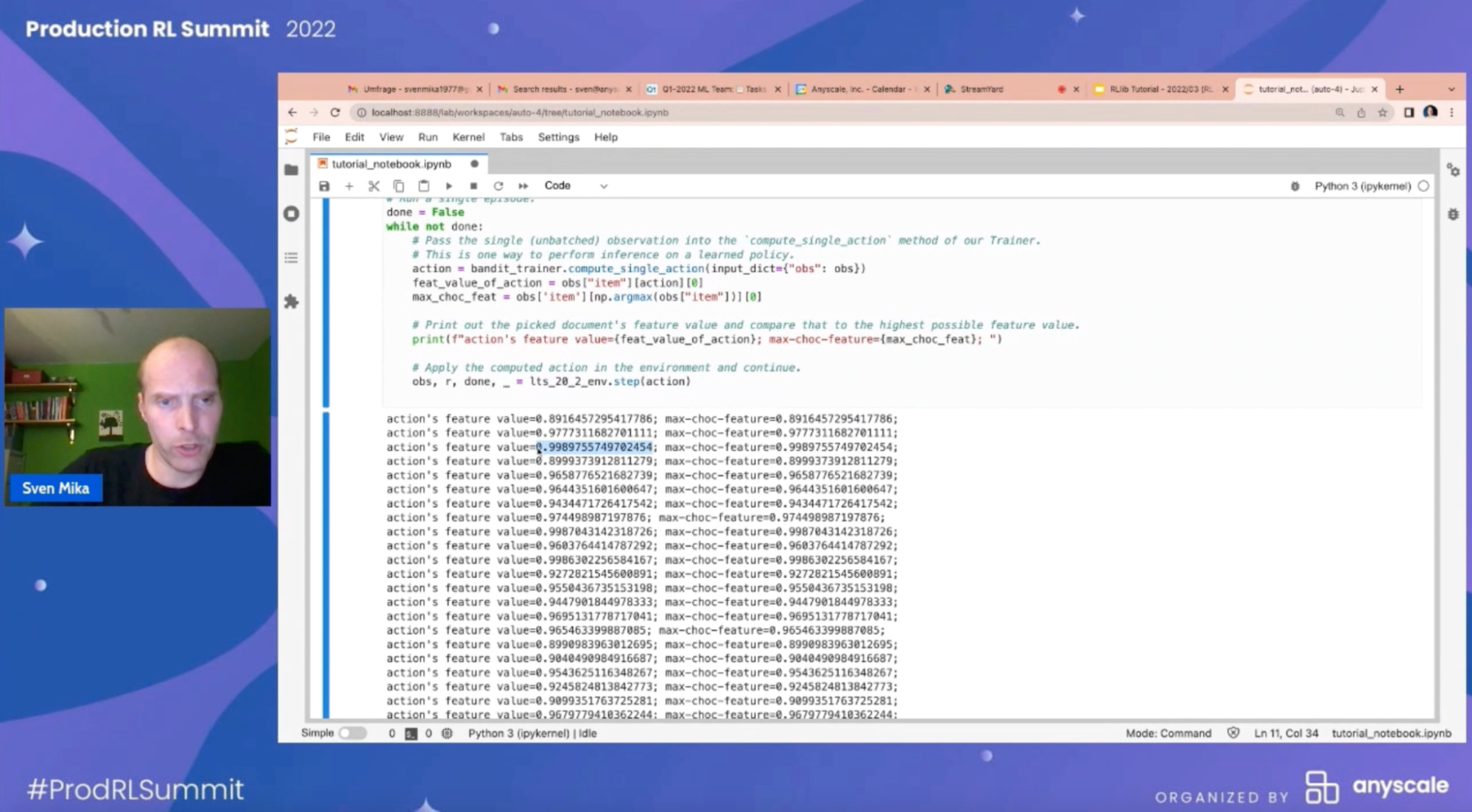
Bandits make each decision independently of past decisions, and they make each decision based on immediate rewards only. In our notebooks, we saw the contextual bandits, when given a choice of 10 products, always chose the product with the highest value in its product feature vector (see image below). This means the optimal value learned from a bandit-run RecSys would always be the maximum immediate reward, not the long-term user satisfaction reward. We also saw from playing around in the notebooks that bandits are extremely sensitive to initial conditions; that is, the final reward the system thinks is possible depends on which recommendations you showed the bandit first.

Contextual bandits always recommend the product with the highest value in its feature embedding vector. A bandit-run recommender system will only recommend immediate reward; it will miss the long-term satisfaction reward.

LinkDeep RL algorithms often have many hyperparameters

The final 30 minutes of the tutorial were spent exploring a Deep RL algorithm with offline RL.  To switch our notebooks away from Bandits:

1. First, we kept the same RecSim environment (with same rewards in short-term feature vectors and hidden state long-term reward per user).  

2. Next, we included user-embedding vectors (user meta-data), since this is a hard requirement of SlateQ in order to personalize a journey for each individual user.  

3. Next, in RLlib, we switched the algorithm from bandit to SlateQ (a deep learning RL algorithm derived from Deep Q-Networks (DQN), developed by the same people at Google that developed RecSim. This algorithm better handles the combinatorial explosion of action choices due to k-slates, and solves for long-term reward which bandits miss).

4. SlateQ has a large number of hyperparameters to tune. Ray Tune was used to find optimal parameter values.

5. The Ray RLlib team maintains a repository of tuned models. These are organized by Algorithm / Environment.yaml. These files are used by the engineering team for daily testing as well as weekly hard-task testing.  This provides a great head-start to tuning your models!

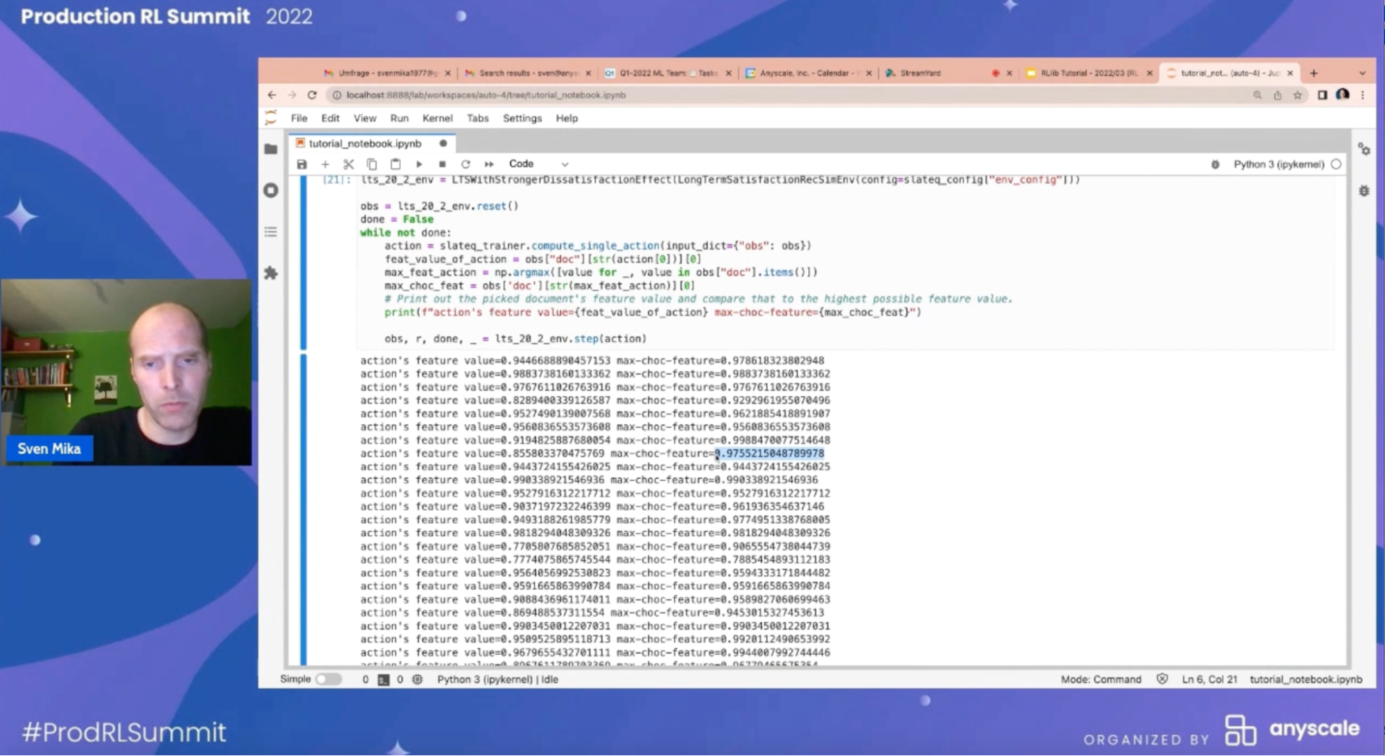
After tuning our RL model, we saw that SlateQ was no longer simply recommending the most click-bait items (see image below). In our small example, mean episode rewards were: 

• Random actions baseline: 1158

• Contextual bandits: 1162 

• SlateQ:  1173

From above rewards (higher is better), we saw that SlateQ gave the best results for multi-objective, long-term rewards, but with the extra effort of hyperparameter tuning. Fortunately, Ray Tune is perfectly integrated with Ray RLlib for exactly this task!

The RL algorithm SlateQ solves for the problems missed by bandits of: a) action space explosion due to k-slates having to be filled with recommendations, and b) inability of bandits to do proper long-term reward assignment.

LinkSeveral classes of algorithms can be used in offline RL

For the offline RL part of the tutorial, we loaded simulation data from a JSON file. Sven explained how you might massage existing, historical interaction data into these JSON files. The simplest offline RL algorithm, behavioral cloning (BC), requires past actions and rewards. If you do not have an environment including rewards, then you also need to supply a formula for “importance sampling” and “weighted importance sampling.” For this part of the tutorial, we used BC, the JSON file, and sampling formulas.

Other offline RL algorithms included in Ray RLlib (CQL, MARWIL, and DQN) consider the offline RL JSON file as pre-trained weights in order to try to learn an even better set of recommendations. These “policy-improving” algorithms need the probabilities of each action to be specified in the JSON file itself. CQL outputs prices as well as product recommendations, which sounds very useful for companies who want to customize their pricing as well as product recommendations. MARWIL, based on BC, is best for discrete action spaces.  

Since RLlib is open source, it is completely modifiable for your needs in either TF2 or PyTorch. (I would love to see a community-contributed modification of DQN adapted to “conservative Q-learning” as described by Sergey Levine in his talk about offline RL).

LinkHow to checkpoint, save, restart and deploy models

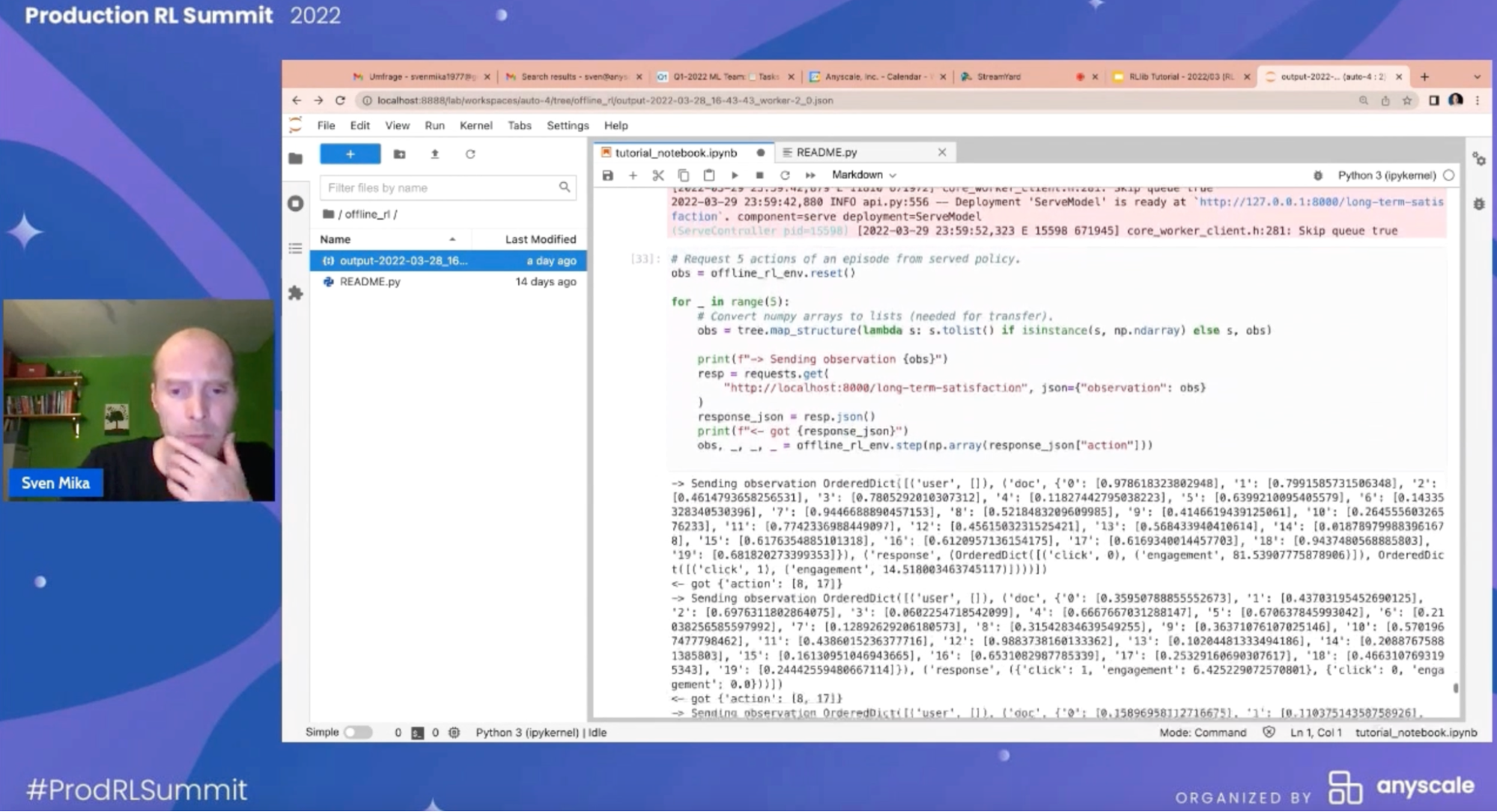
To finish off the tutorial, Sven showed us how to deploy RL models using Ray Serve. First, we saw how to save training checkpoint files, then load those files and warm restart training using RLlib’s trainer.restore(). Finally, we saw a quick example of how to use Ray Serve’s Python decorator @serve.deployment(route_prefix) to convert any regular Python class to serve already-trained models on an endpoint, reachable at my_server:8000/route_prefix. This allows you to serve RL (or any kind of ML model) for inference, in production, in a distributed fashion, using Ray Serve.

Next, we are presenting at the ODSC-East conference in Boston. I’m really looking forward to meeting people there!

Deploying a model-serving distributed endpoint using Ray Serve.

If you’d like to hear more and keep in touch with the Ray RLlib team: 

• Ray forums: discuss.ray.io/

• Slack us on: #rllib channel on ray-distributed.slack.com

• File an issue, contribute, give us a star 🙂 github.com/ray-project/ray/tree/master/rllib