How continuous batching enables 23x throughput in LLM inference while reducing p50 latency
In this blog, we’ll cover the basics of large language model (LLM) inference and highlight inefficiencies in traditional batching policies. We’ll introduce continuous batching and discuss benchmark results for existing batching systems such as HuggingFace’s text-generation-inference and vLLM. By leveraging vLLM, users can achieve 23x LLM inference throughput while reducing p50 latency.
Due to the large GPU memory footprint and compute cost of LLMs, serving dominates the compute cost for most real world applications. ML engineers often treat LLMs like "black boxes" that can only be optimized with internal changes such as quantization and custom CUDA kernels. However, this is not entirely the case. Because LLMs iteratively generate their output, and because LLM inference is often memory and not compute bound, there are surprising system-level batching optimizations that make 10x or more differences in real-world workloads.
One recent such proposed optimization is continuous batching, also known as dynamic batching, or batching with iteration-level scheduling. We wanted to see how this optimization performs. We will get into details below, including how we simulate a production workload, but to summarize our findings:
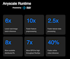
Up to 23x throughput improvement using continuous batching and continuous batching-specific memory optimizations (using vLLM).
8x throughput over naive batching by using continuous batching (both on Ray Serve and Hugging Face’s text-generation-inference).
4x throughput over naive batching by using an optimized model implementation (NVIDIA’s FasterTransformer).
You can try out continuous batching today: see this example to run vLLM on Ray Serve.
The remainder of this blog is structured as follows:
We’ll cover the basics of how LLM inference works and highlight inefficiencies in traditional request-based dynamic batching policies.
We’ll introduce continuous batching and how it answers many of the inefficiencies of request-based dynamic batching.
We then discuss our benchmarks and the implications this has on how to serve LLM models cost-effectively.
LinkThe basics of LLM inference
There is a lot to know about LLM inference, and we refer users to Efficient Inference on a Single GPU and Optimization story: Bloom inference for more detail. However, at a high level, LLM inference is pretty straightforward.
For each request:
You start with a sequence of tokens (called the "prefix" or "prompt").
The LLM produces a sequence of completion tokens, stopping only after producing a stop token or reaching a maximum sequence length.
This is an iterative process. You get one additional completion token for each new forward pass of the model. For example, suppose you prompt with a sentence "What is the capital of California: ", it would take ten forward pass iterations to get back the full response of ["S", "a", "c", "r", “a”, "m", "e", "n", "t", "o"]. This example simplifies things a little bit because in actuality tokens do not map 1:1 to ASCII characters (a popular token encoding technique is Byte-Pair Encoding which is beyond the scope of this blog post), but the iterative nature of generation is the same regardless of how you tokenize your sequences.
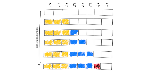 Simplified LLM inference. This toy example shows a hypothetical model which supports a maximum sequence length of 8 tokens (T1, T2, …, T8). Starting from the prompt tokens (yellow), the iterative process generates a single token at a time (blue). Once the model generates an end-of-sequence token (red), the generation loop stops. This example shows a batch of only one input sequence, so the batch size is 1.
Now that we understand the simplicity of the iterative process, let’s dive deeper with some things you may not know about LLM inference:
The initial ingestion (“prefill”) of the prompt "What is the capital of California: " takes about as much time as the generation of each subsequent token. This is because the prefill phase pre-computes some inputs of the attention mechanism that remain constant over the lifetime of the generation. This prefill phase efficiently uses the GPU’s parallel compute because these inputs can be computed independently of each other.
LLM inference is memory-IO bound, not compute bound. In other words, it currently takes more time to load 1MB of data to the GPU’s compute cores than it does for those compute cores to perform LLM computations on 1MB of data. This means that LLM inference throughput is largely determined by how large a batch you can fit into high-bandwidth GPU memory. See this page in the NVIDIA docs for more details.
The amount of GPU memory consumed scales with the base model size + the length of the token sequence. In Numbers every LLM developer should know, it’s estimated that a 13B parameter model consumes nearly 1MB of state for each token in a sequence. On a higher-end A100 GPU with 40GB RAM, back-of-the-envelope math suggests that since 14 GB are left after storing the 26GB of model parameters, ~14k tokens can be held in memory at once. This may seem high but is actually quite limiting; if we limit our sequence lengths to 512, we can process at most ~28 sequences in a batch. The problem is worse for higher sequence lengths; a sequence length of 2048 means our batch size is limited to 7 sequences. Note that this is an upper bound since it doesn’t leave room for storing intermediate computations.
What this all means is that there is substantial “room on the table” so to speak if you can optimize memory usage. This is why approaches such as model quantization strategies such as AutoGPTQ are potentially so powerful; if you could halve the memory usage by moving from 16-bit to 8-bit representations, you could double the space available for larger batch sizes. However, not all strategies require modifications to the model weights. For example, FlashAttention found significant throughput improvements by reorganizing the attention computation to require less memory-IO.
Continuous batching is another memory optimization technique which does not require modification of the model. We next explain how naive batching works (and is inefficient), and how continuous batching increases the memory-efficiency of LLM generation.
LinkLLM batching explained
GPUs are massively-parallel compute architectures, with compute rates (measured in floating-point operations per second, or flops) in the teraflop (A100) or even petaflop (H100) range. Despite these staggering amounts of compute, LLMs struggle to achieve saturation because so much of the chip’s memory bandwidth is spent loading model parameters.
Batching is one way to improve the situation; instead of loading new model parameters each time you have an input sequence, you can load the model parameters once and then use them to process many input sequences. This more efficiently uses the chip’s memory bandwidth, leading to higher compute utilization, higher throughput, and cheaper LLM inference.
LinkNaive batching / static batching
We call this traditional approach to batching static batching, because the size of the batch remains constant until the inference is complete. Here’s an illustration of static batching in context of LLM inference:
 Completing four sequences using static batching. On the first iteration (left), each sequence generates one token (blue) from the prompt tokens (yellow). After several iterations (right), the completed sequences each have different sizes because each emits their end-of-sequence-token (red) at different iterations. Even though sequence 3 finished after two iterations, static batching means that the GPU will be underutilized until the last sequence in the batch finishes generation (in this example, sequence 2 after six iterations).
Unlike traditional deep learning models, batching for LLMs can be tricky due to the iterative nature of their inference. Intuitively, this is because requests can "finish" earlier in a batch, but it is tricky to release their resources and add new requests to the batch that may be at different completion states. This means that as the GPU is underutilized as generation lengths of different sequences in a batch differ from the largest generation length of the batch. In the figure on the right above, this is illustrated by the white squares after end-of-sequence tokens for sequences 1, 3, and 4.
How often does static batching under-utilize the GPU? It depends on the generation lengths of sequences in a batch. For example, one could use LLM inference to emit a single token as a classification task (there are better ways to do this but let’s use this as an example). In this case, every output sequence is the same size (1 token). If the input sequences are also the same size (say, 512 tokens), then each static batch will achieve the best possible GPU utilization.
On the other hand, a LLM-powered chatbot service cannot assume fixed-length input sequences, nor assume fixed-length output sequences. Proprietary models offer maximum context lengths in excess of 8K tokens at the time of writing. With static batching, variance in generation output could cause massive underutilization of GPUs. It’s no wonder OpenAI CEO Sam Altman described the compute costs as eye-watering.
Without restrictive assumptions on user input and model output, unoptimized production-grade LLM systems simply can’t serve traffic without underutilizing GPUs and incurring unnecessarily high costs. We need to optimize how we serve LLMs for their power to be broadly accessible.
LinkContinuous batching
The industry recognized the inefficiency and came up with a better approach. Orca: A Distributed Serving System for Transformer-Based Generative Models is a paper presented in OSDI ‘22 which is the first to our knowledge to tackle this problem. Instead of waiting until every sequence in a batch has completed generation, Orca implements iteration-level scheduling where the batch size is determined per iteration. The result is that once a sequence in a batch has completed generation, a new sequence can be inserted in its place, yielding higher GPU utilization than static batching.
 Completing seven sequences using continuous batching. Left shows the batch after a single iteration, right shows the batch after several iterations. Once a sequence emits an end-of-sequence token, we insert a new sequence in its place (i.e. sequences S5, S6, and S7). This achieves higher GPU utilization since the GPU does not wait for all sequences to complete before starting a new one.
Reality is a bit more complicated than this simplified model: since the prefill phase takes compute and has a different computational pattern than generation, it cannot be easily batched with the generation of tokens. Continuous batching frameworks currently manage this via hyperparameter: waiting_served_ratio, or the ratio of requests waiting for prefill to those waiting end-of-sequence tokens.
Speaking of frameworks, Hugging Face has productionized continuous batching in their Rust- and Python-based text-generation-inference LLM inference server. We use their implementation to understand the performance characteristics of continuous batching in our benchmarks below.
Note: Continuous batching, dynamic batching, and iteration-level scheduling are all close enough in meaning that any one of them can be used to describe the batching algorithm. We chose to use continuous batching. Dynamic batching is fitting but can be confused with request-level batching, where an LLM inference server uses a static batch whose size is chosen when the current batch has completely finished generation. We feel that iteration-level scheduling is descriptive of the scheduling mechanism but not the process as a whole.
LinkPagedAttention and vLLM
For this blog post, we want to showcase the differences between static batching and continuous batching. It turns out that continuous batching can unlock memory optimizations that are not possible with static batching by improving upon Orca’s design.
PagedAttention is a new attention mechanism implemented in vLLM (GitHub). It takes inspiration from traditional OS concepts such as paging and virtual memory. They allow the KV cache (what is computed in the “prefill” phase, discussed above) to be non-contiguous by allocating memory in fixed-size “pages”, or blocks. The attention mechanism can then be rewritten to operate on block-aligned inputs, allowing attention to be performed on non-contiguous memory ranges.
This means that buffer allocation can happen just-in-time instead of ahead-of-time: when starting a new generation, the framework does not need to allocate a contiguous buffer of size maximum_context_length. Each iteration, the scheduler can decide if it needs more room for a particular generation, and allocate on the fly without any degradation to PagedAttention’s performance. This doesn’t guarantee perfect utilization of memory (their blog says the wastage is now limited to under 4%, only in the last block), but it significantly improves upon wastage from ahead-of-time allocation schemes used widely by the industry today.
Altogether, PagedAttention + vLLM enable massive memory savings as most sequences will not consume the entire context window. These memory savings translate directly into a higher batch size, which means higher throughput and cheaper serving. We include vLLM in our benchmarks below.
LinkBenchmarking setup
We’ll discuss our experimental setup then dive into the results of our benchmarks.
LinkExperiments
Our goal is to see how continuous batching performs versus static batching on a simulated real-world live-inference workload. Fundamentally, we care about cost. We break this down into throughput and latency since cost is directly downstream of how efficiently you can serve at a given latency.
Benchmark goal | Measurement |
Measure throughput | Time-to-process a queue of 1000 requests, each with 512 input tokens and generation length sampled from an exponential distribution. |
Measure latency | Request latencies for 100 requests, with varying input lengths, output lengths, and arrival times at a fixed average rate. |
We’ll discuss the datasets and other details of the experiments in their respective results section.
LinkHardware/model
We benchmark throughput and latency on a single NVIDIA A100 GPU provided by Anyscale. Our A100 has 40GB of GPU RAM. We selected Meta’s OPT-13B model because each framework under test had a readily-available integration with this model. We selected the 13B variant because it fits into our GPU without requiring tensor parallelism, yet is still large enough to present memory efficiency challenges. We opt not to use tensor parallelism, where each transformer block is split over multiple GPUs, to keep our experiments simple, although both static batching and continuous batching work with tensor parallelism.
LinkFrameworks

We test two static batching frameworks and three continuous batching frameworks. Our static batching frameworks are:
Hugging Face’s Pipelines. This is the simplest inference solution. It provides static batching with an easy-to-use API that works with any model and supports more tasks than simple text-generation. We use this as our baseline.
NVIDIA’s FasterTransformer. This is a library which provides optimized implementations of various transformer models. It currently only provides static batching (the Triton inference server provides request-level dynamic batching, but not continuous batching yet). This provides us with an idea of how far an extremely optimized implementation of our model can get us with static batching – it provides a more competitive baseline than the relatively unoptimized OPT-13B implementation available on Hugging Face Hub.
Our continuous batching frameworks are:
Hugging Face’s text-generation-inference. This is the inference server Hugging Face uses to power their LLM live-inference APIs. It implements continuous batching.
Continuous batching on Ray Serve. Ray Serve leverages Ray’s serverless capabilities to provide seamless autoscaling, high-availability, and support for complex DAGs. We wanted to understand how continuous batching works, so we re-implemented text-generation-inference’s core continuous batching logic in pure-Python on Ray Serve. As you will see in our results, our implementation achieves the same performance as text-generation-inference, which validates our understanding.
vLLM. This is an open-source project recently released by folks at UC Berkeley (GitHub). It builds upon Orca’s continuous batching design by taking full control of dynamic memory allocations, allowing it to significantly reduce different forms of GPU memory fragmentation. We test this framework because it shows the impact of further optimizations made possible by iteration-level scheduling and continuous batching.
LinkBenchmarking results: Throughput
Based on our understanding of static batching, we expect continuous batching to perform significantly better when there is higher variance in sequence lengths in each batch. To show this, we run our throughput benchmark four times for each framework, each time on a dataset with higher variance in sequence lengths.
To do this, we create a dataset containing 1000 sequences each with 512 input tokens. We configure our model to always emit a per-sequence generation length by ignoring the end-of-sequence token and configuring max_tokens. We then generate 1000 generation lengths, one for each request, sampled from an exponential distribution with mean=128 tokens. We use an exponential distribution as it is a good approximation of the generation lengths that one may encounter while serving an application like ChatGPT. To vary the variance of each run, we select only samples from the exponential distribution that are less than or equal to 32, 128, 512, and 1536. The total output sequence length is then, at most, 512+32=544, 512+128=640, 512+512=1024, and 512+1536=2048 (the maximum sequence length of our model).
We then use a simple asyncio Python benchmarking script to submit HTTP requests to our model server. The benchmarking script submits all requests in burst fashion, so that the compute is saturated.
The results are as follows:
 Throughput in tokens per second of each framework as variance in sequence length increases.
As expected, the static batchers and naive continuous batchers perform approximately identically for lower-variance generation lengths. However as the variance increases, naive static batching’s performance plummets to 81 token/s. FasterTransformers improves upon naive static batching significantly, nearly keeping up with the naive continuous batchers until generation length limit of 1536. Continuous batching on Ray Serve and text-generation-inference achieves about the same performance, which is what we expect since they use the same batching algorithm.
What is most impressive here is vLLM. For each dataset, vLLM more than doubles performance compared to naive continuous batching. We have not analyzed what optimization contributes the most to vLLM performance the most, but we suspect vLLM’s ability to reserve space dynamically instead of ahead-of-time allows vLLM to dramatically increase the batch size.
We plot these performance results relative to naive static batching:
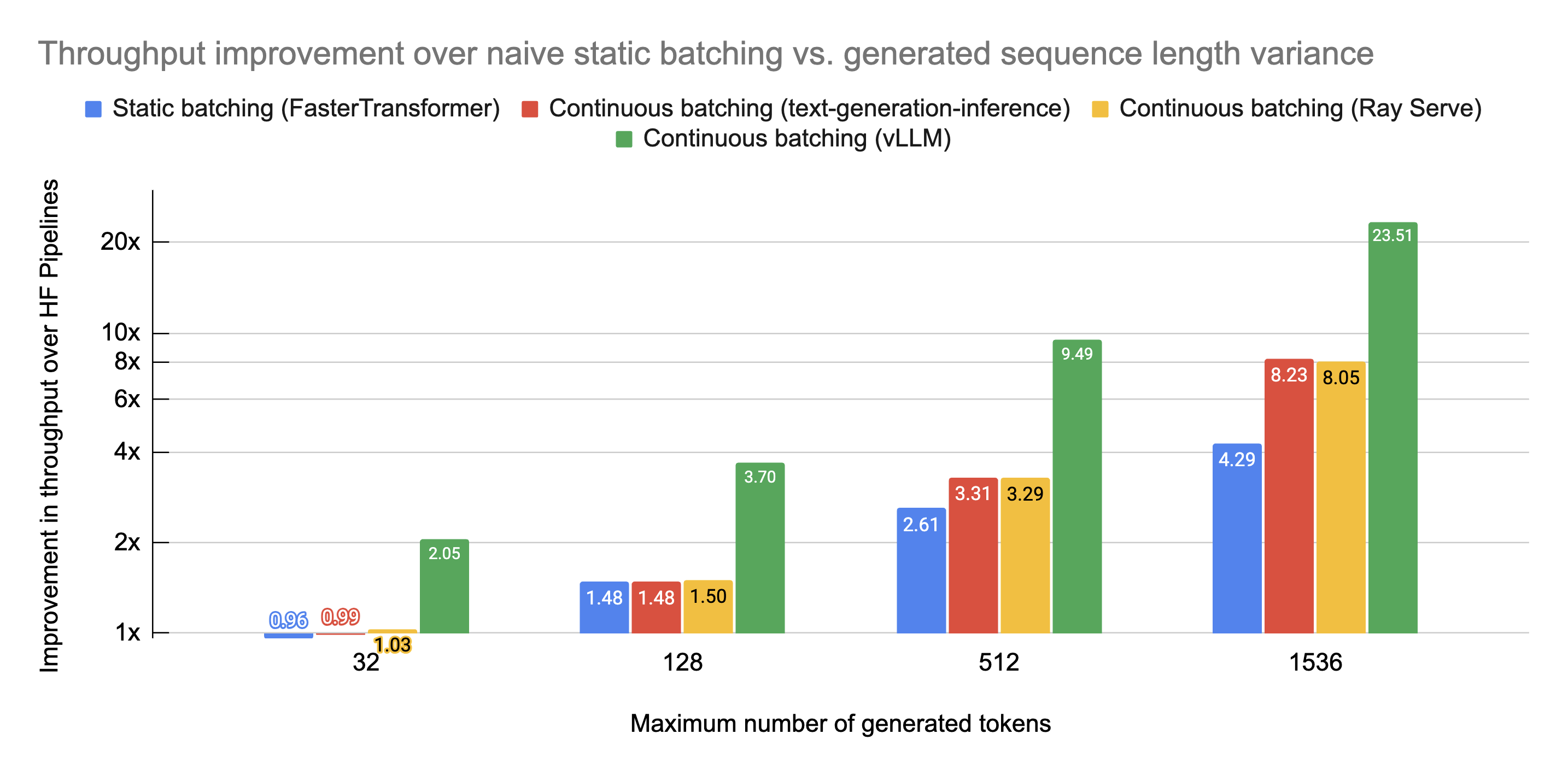 Our throughput benchmark results presented as improvement multiples over naive static batching, log scale.
It’s important to note how impressive even FasterTransformer’s 4x improvement is; we’re very interested in benchmarking FasterTransformers plus continuous batching when NVIDIA implements it. However, continuous batching is clearly a significant improvement over static batching even with an optimized model. The performance gap becomes gigantic when you include further memory optimization enabled by continuous batching and iteration-level scheduling as vLLM does.
LinkBenchmarking results: Latency
Live-inference endpoints often face latency-throughput tradeoffs that must be optimized based on user needs. We benchmark latency on a realistic workload and measure how the cumulative distribution function of latencies changes with each framework.
Similar to the throughput benchmark, we configure the model to always emit a specified amount of tokens specified per-request. We prepare 100 randomly-generated prompts by sampling lengths from a uniform distribution between 1 token and 512 tokens. We sample 100 output lengths from a capped exponential distribution with mean=128 and maximum size of 1536. These numbers were chosen because they are reasonably realistic and allow the generation to use up the full context-length of our model (512+1536=2048).
Instead of submitting all requests at the same time as done in the throughput benchmark, we delay each request by a predetermined number of seconds. We sample a Poisson distribution to determine how long each request waits after the previously submitted request. The Poisson distribution is parameterized by λ, the expected rate, which in our case is how many queries per second (QPS) hit our model endpoint. We measure latencies at both QPS=1 and QPS=4 to see how the latency distribution changes as load changes.
 Median generation request latency for each framework, under average load of 1 QPS and 4 QPS. Continuous batching systems improve median latency.
We see that while improving throughput, continuous batching systems also improve median latency. This is because continuous batching systems allow for new requests to be added to an existing batch if there is room, each iteration. But how about other percentiles? In fact, we find that they improve latency across all percentiles:
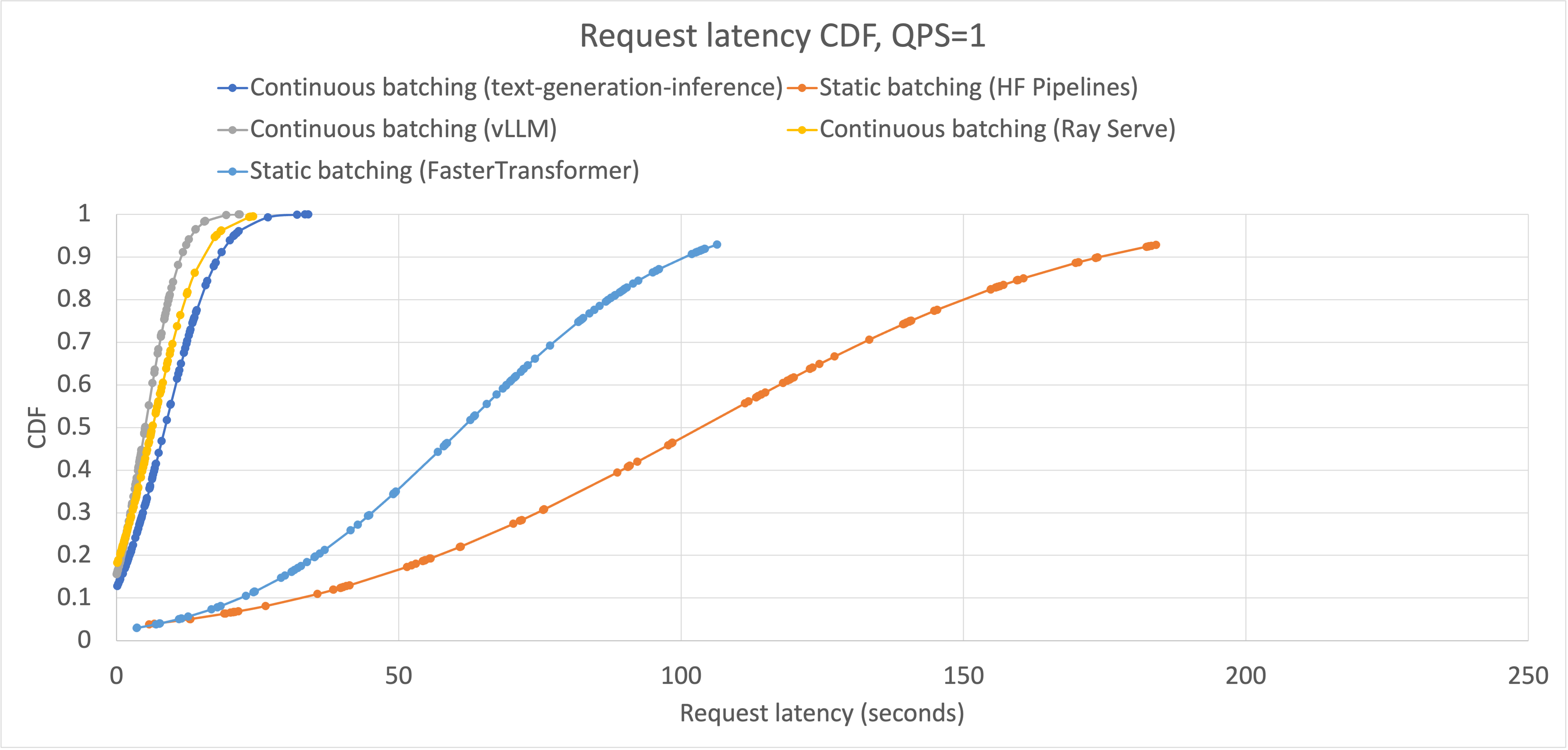 Cumulative distribution function of generation request latencies for each framework with QPS=1. Static batchers and continuous batchers have distinct curve shapes caused by the presence of iteration-level batch scheduling in continuous batchers. All continuous batchers perform approximately equally under this load; FasterTransformers performs noticeably better than static batching on a naive model implementation.
The reason why continuous batching improves latency at all percentiles is the same as why it improves latency at p50: new requests can be added regardless of how far into generation other sequences in the batch are. However, like static batching, continuous batching is still limited by how much space is available on the GPU. As your serving system becomes saturated with requests, meaning a higher on-average batch size, there are less opportunities to inject new requests immediately when they are received. We can see this as we increase the average QPS to 4:
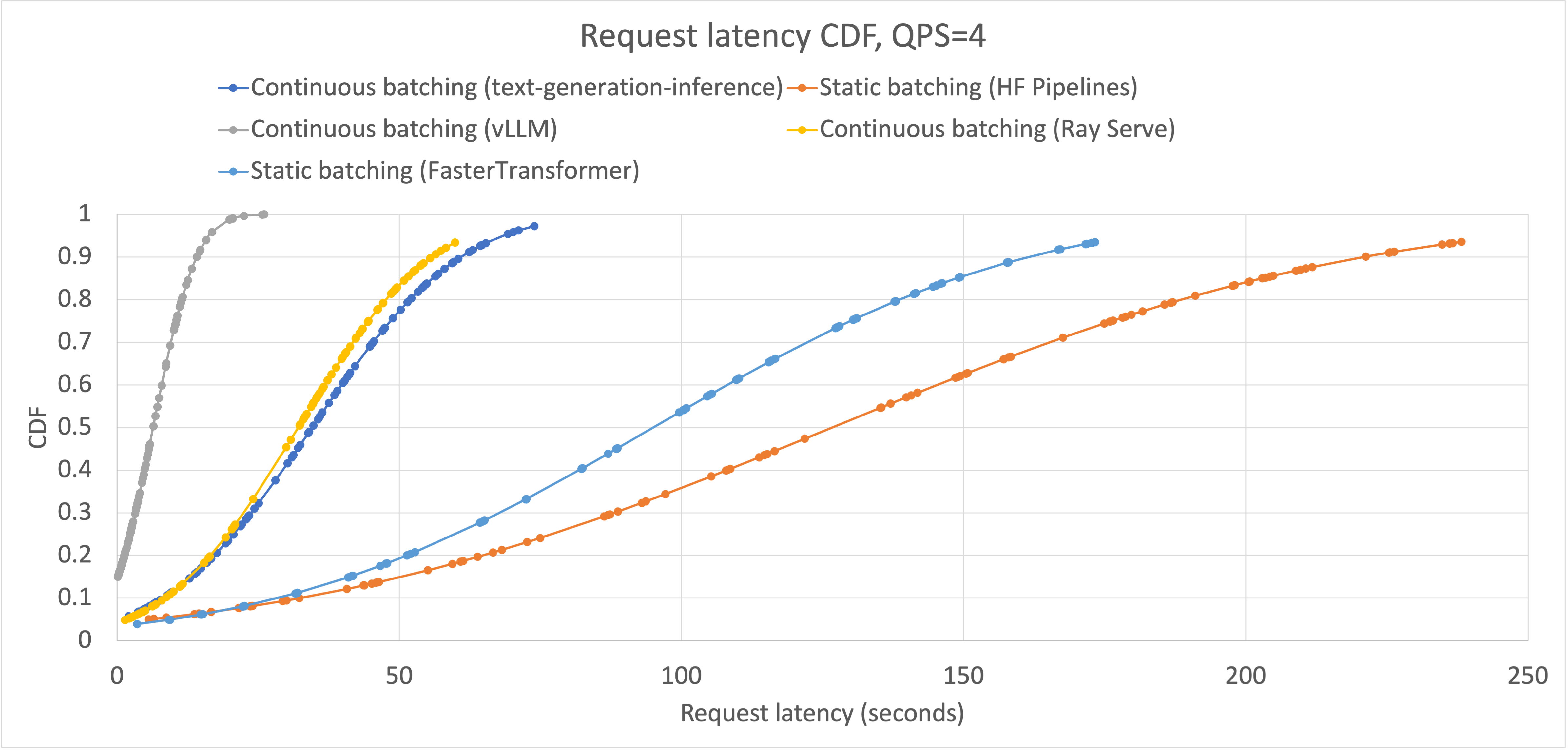 Cumulative distribution function of generation request latencies for each framework with QPS=4. Compared to QPS=1, FasterTransformer’s distribution of latencies becomes more similar to static batching on a naive model. Both Ray Serve and text-generation-inference’s continuous batching implementations perform similarly, but noticeably worse than vLLM.
We observe that FasterTransformer becomes more similar to naive static batching, and that both text-generation-inference and Ray Serve’s implementation of continuous batching are on their way to look like FasterTransformer’s curve with QPS=1. That is, as the systems become saturated there are less opportunities to inject new requests immediately, so request latency goes up. This lines up with the vLLM curve – it remains mostly unchanged between QPS=1 and QPS=4. This is because due to its advanced memory optimizations, it has a higher maximum batch size.
Anecdotally, we observe that vLLM becomes saturated around QPS=8 with a throughput near 1900 token/s. To compare these numbers apples-to-apples to the other serving systems requires more experimentation; however we have shown that continuous batching significantly improves over static batching by 1) reducing latency by injecting new requests immediately when possible, and 2) enable advanced memory optimizations (in vLLM’s case) that increase the QPS that the serving system can handle before becoming saturated.
LinkConclusion
LLMs present some amazing capabilities, and we believe their impact is still mostly undiscovered. We have shared how a new serving technique, continuous batching, works and how it outperforms static batching. It improves throughput by wasting fewer opportunities to schedule new requests, and improves latency by being capable of immediately injecting new requests into the compute stream. We are excited to see what people can do with continuous batching, and where the industry goes from here.
LinkTry out continuous batching for yourself
We have a vLLM + Ray Serve example that allows you to try out continuous batching. We are integrating continuous batching systems into Aviary, a webapp that allows you to compare the outputs of different LLMs in parallel, and will release it within the week.
Acknowledgements. We’d like to thank the following people for assisting in benchmarking and/or reviewing our results. Anyscale: Stephanie Wang, Antoni Baum, Edward Oakes, and Amog Kamsetty; UC Berkeley: Zhuohan Li and Woosuk Kwon.
LinkGet involved with Ray
The code used for the experiments in the blog post is here. To connect with the Ray community, join the Ray Slack or ask questions on the Discuss forum. If you are interested in hosting LLMs, check out our managed Ray offering. If you are interested in learning more about Ray, see ray.io and docs.ray.io.
See our earlier blog series on solving Generative AI infrastructure and using LangChain with Ray.
Ray Summit 2023: If you are interested to learn much more about how Ray can be used to build performant and scalable LLM applications and fine-tune/train/serve LLMs on Ray, join Ray Summit on September 18-20th! We have a set of great keynote speakers including John Schulman from OpenAI and Aidan Gomez from Cohere, community and tech talks about Ray as well as practical training focused on LLMs.
Table of contents
- The basics of LLM inference
- LLM batching explained
- Naive batching / static batching
- Continuous batching
- PagedAttention and vLLM
- Benchmarking setup
- Experiments
- Hardware/model
- Frameworks
- Benchmarking results: Throughput
- Benchmarking results: Latency
- Conclusion
- Try out continuous batching for yourself
- Get involved with Ray
