Link1. Introduction

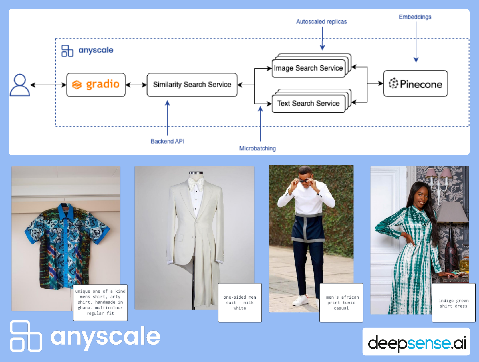
Motivated by the emerging trend of multimodality, deepsense.ai teamed up with Anyscale to develop a fashion image retrieval system that serves as a reference for those looking to build similar applications. Our implementation's modular and service-oriented design allows for easy reuse of our code for custom data and tasks, while also providing an optimal approach for scalability.

Throughout this guide, we will walk you through the step-by-step process of:

• Utilizing the Contrastive Language-Image Pre-training (CLIP) models, both general-domain and domain-specific, to obtain text and image embeddings

• Building vector indices for text and image embeddings with Pinecone

• Embedding input text or images on the fly during online inference

• Harnessing Ray Data for efficient and distributed data processing

• Building a scalable application for cross-modal image retrieval with Anyscale Services.

By the end of this guide, you will have developed a comprehensive application with a scalable and performant backend and a fully operational interface. This interface allows users to search seamlessly for images within the dataset using text or image prompts. We will also share insights comparing the use of a standard CLIP model to a fine-tuned, domain-specific one, discussing the advantages of each approach.

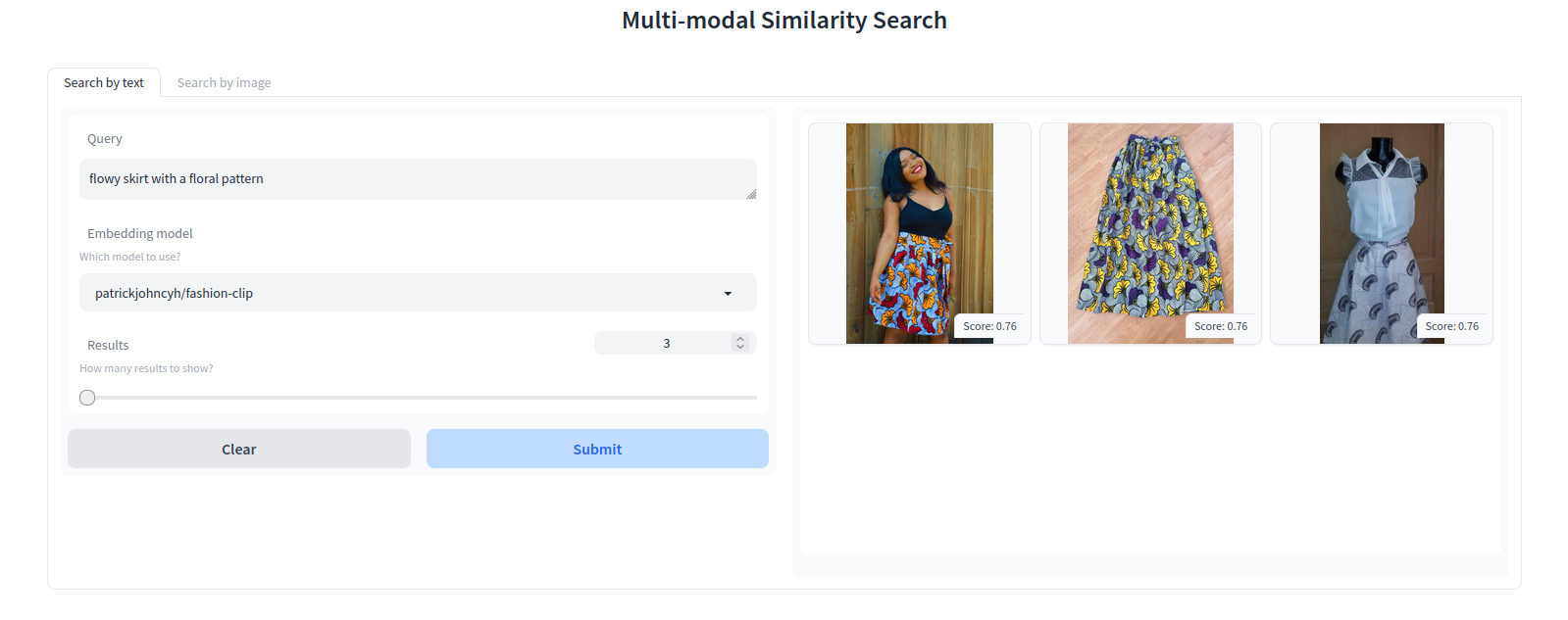Fig. 1 Application frontend view. Results for the prompt “flowy skirt with a floral pattern”.

Link2. Application overview

In the e-commerce world, the search for the perfect purchase can be challenging. With numerous product pages to sift through, searching by a product's description or name alone is often insufficient due to the varying quality and sophistication of product metadata. We often seek items we have seen before, such as a dress worn by a favorite influencer or a home decor piece from a TV show.

The desire to find similar items drives the search for visually comparable products. This is where the capability to perform text-to-image and image-to-image searches becomes valuable. Simply describe the item or upload the image into the search bar! Image retrieval systems based on CLIP embeddings can combine textual descriptions with visual data in one space, leading to more intuitive and accurate searches that bridge the gap between user intent and available inventory.

Let's explore the core components of our app:

• An end-to-end scalable embeddings generation data pipeline

• A scalable backend providing a retrieval system powered by

  • A self-hosted CLIP embeddings model, ensuring sensitive data remains secure

  • Vector similarity search using Pinecone as the vector database

• A sleek and intuitive Gradio frontend

In the app, users can select their preferred embedding model, adjust the number of images for retrieval, and input outfit descriptions or upload images. These features ensure users can effortlessly find visually similar items, enhancing their overall experience. The result is that the user receives N images from the dataset that most closely match their query, based on cosine similarity.

Link3. Multi-modal embeddings

In this section, we will guide you through creating the vector store and generating embeddings. We will also provide some insight into how the CLIP model functions.

Before the creation of the application, we need to process and load our documents into a vector search index. This includes the following steps:

1. Prepare the dataset, including images and their descriptions (in our case, the InFashAIv1 dataset).

2. Use CLIP to generate text embeddings (embedded text descriptions) and image embeddings.

3. Use Pinecone to create a vector database for storing the embeddings.

Link3.1 CLIP models 

OpenAI introduced the original CLIP model in 2021, with details described in their blog post "CLIP: Connecting text and images". Given a set of N (image, text) pairs, the CLIP model is trained to identify the actual pairings within the batch among N × N potential combinations. This training objective leads to the creation of a multi-modal embedding space.

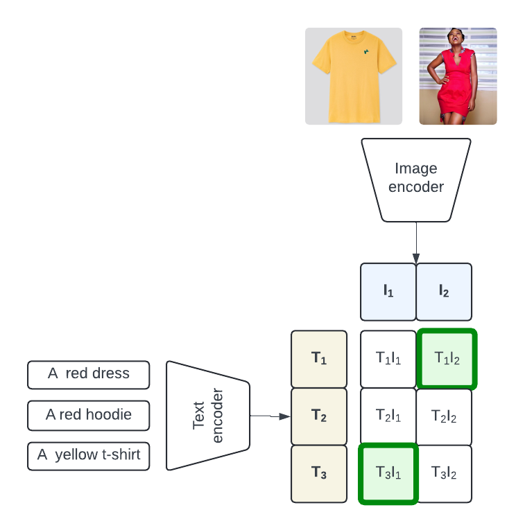Fig.2 Overview of the CLIP model architecture. CLIP maximizes the similarity score between correct pairs of <image, text description> (marked here in green). Image by the authors, images from InFashAIv1 dataset.

The process involves:

1. Training an image encoder and a text encoder.

2. Increasing the cosine similarity of embeddings for the correct pairs.

3. Decreasing the cosine similarity for the incorrect pairings.

It is important to note that CLIP is not a generative model; it does not create text snippets or images. Instead, it uses the embedding space to compute a semantic similarity score between a text and image.

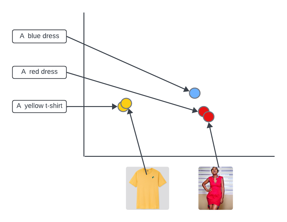Fig. 3 CLIP embeds images and text descriptions in the same vector space. If you have an image, you can easily search for the caption. If you have text, you can search for the closest description. Image by the authors, using images from InFashAIv1 dataset.

OpenAI released the first CLIP model, but others have created their versions by fine-tuning them on different datasets, altering hyperparameters, or changing the encoders. An example is OpenCLIP by LAION.

Link3.2 Domain-specific CLIP

While general CLIP models offer broad capabilities, there are times when the need to fine-tune a custom one arises. Off-the-shelf models may not fully capture the nuances of specialized tasks or domains, such as medical, remote sensing, or fashion.

To create a custom CLIP tailored to your needs, you might:

• Fine-tune it on a custom, domain-specific dataset.

• Modify or adjust the model's architecture.

Some examples include:

1. RemoteCLIP - a vision-language foundation model for remote sensing, tuned using in-domain aerial imagery data.

2. BiomedCLIP - a specialized model trained with fifteen million scientific image-text pairs, where the authors incorporated a domain-specific language model (PubMedBERT) and adjusted tokenizers and context sizes to align with the characteristics of biomedical images and texts.

3. FashionCLIP - a vision and language model for the fashion industry, which is the result of finetuning LAION OpenCLIP with 700K <image, caption> pairs, with images of products from the Farfetch website.

Our application supports two models: the original OpenAI CLIP and FashionCLIP. This allows us to explore the differences in performance between general-purpose and in-domain models, which we cover in section 5 of this guide.

Link3.3 Dataset overview

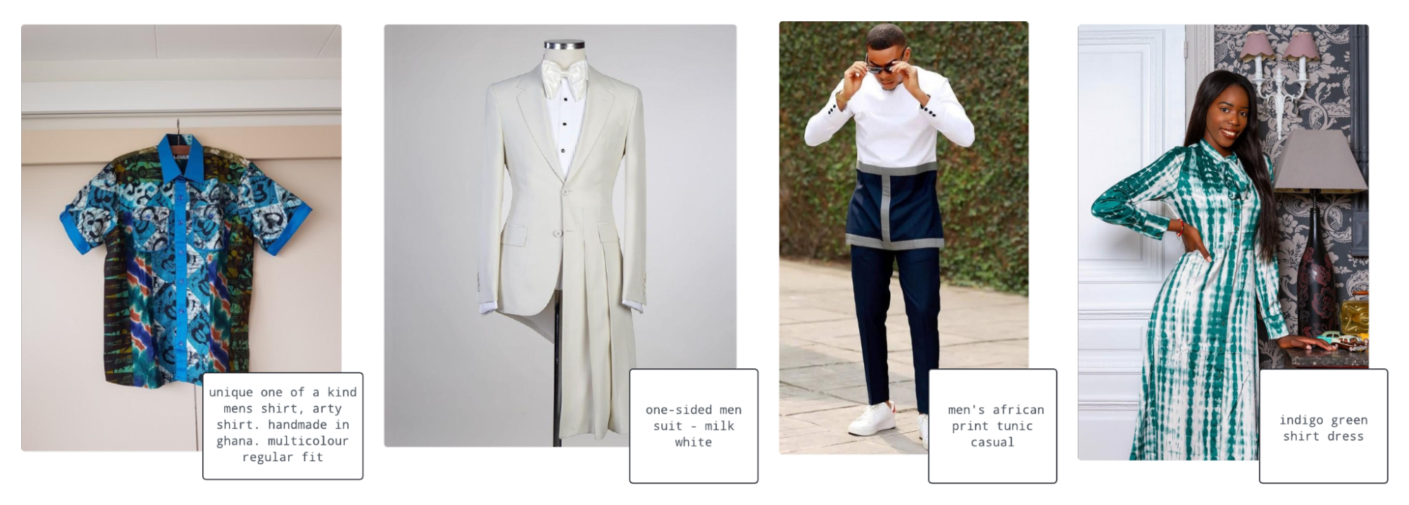Fig. 4 Sample images and captions from the InFashAIv1 dataset. The dataset contains pictures of unique clothes, with extraordinary fit and patterns, which can pose a challenge for a model trained on dissimilar or more prevalent datasets.

InFashAIv1 is a dataset introduced in 2021 in the paper “Neural Fashion Image Captioning: Accounting for Data Diversity” by Gilles Hacheme and Noureini Sayouti, and published publicly on Github. It is distinctive for its focus on African fashion, which presents an additional challenge for general-purpose models as most popular fashion-related datasets do not include such diverse outfits. It consists of more than 15,000 images and their annotations in the form of detailed item descriptions.

We have modified the image descriptions to make them more suitable for our use case. We removed all but the outfit summary, leaving the name of the clothes, the fit style, and the color (see the example descriptions in Figure 4 above).

Link3.4 A Scalable data pipeline with Ray Data

Here is a high-level overview of the distributed process of embedding generation we implemented:

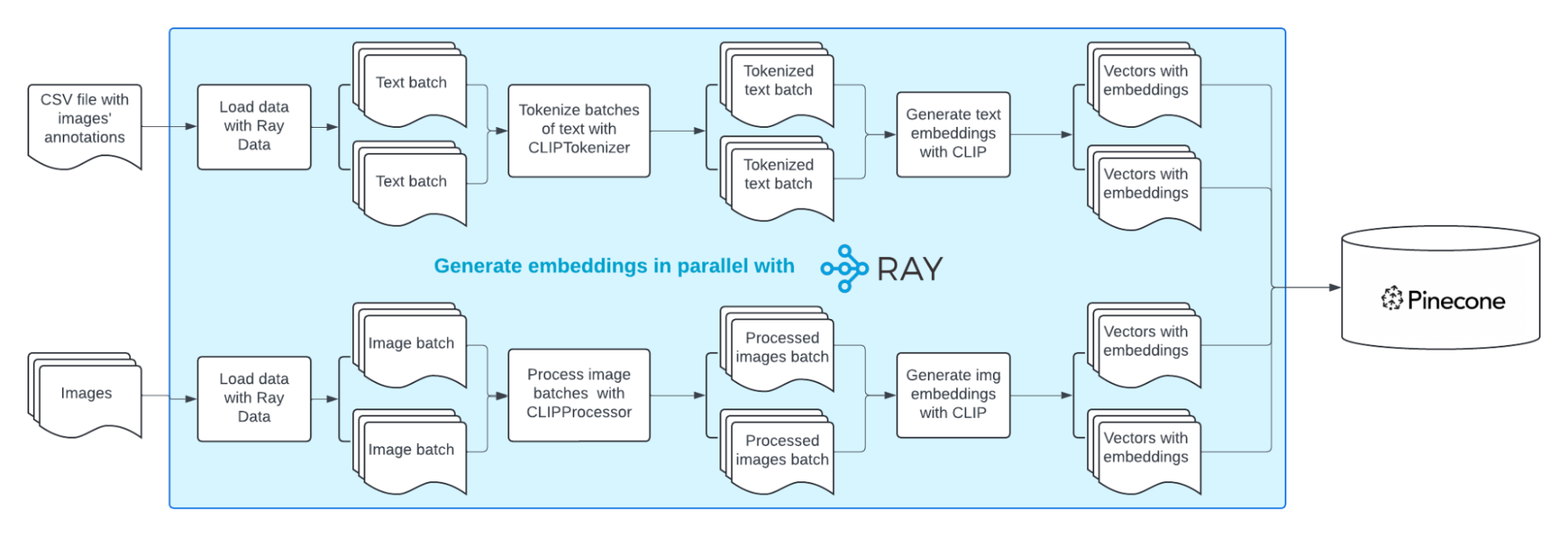
Let's examine it in detail:

1. Data ingestion: We load the image and text data from S3 using Ray Data's IO functionality.

2. Data processing: We applied the following distributed transformations to our lazily loaded Ray Dataset:

   1. Tokenized text descriptions with CLIPTokenizer,

   2. Processed images with CLIPProcessor.

3. Embedding generation: We employed CLIPModel to obtain image and text embeddings. Ray Data’s streaming execution will continuously pass processed image and token blocks to a distributed pool of CLIP model instances.

4. Data postprocessing: We create Pinecone compatible vectors.

5. Vector upserting: Utilizing Ray Data, we upsert the batches of vectors into the Pinecone vector database

 CLIPModel and CLIPProcessor are the main components of the CLIP implementation we used:

• CLIPModel is the core neural network model that powers the CLIP architecture

• CLIPProcessor serves as a wrapper that combines both the CLIPImageProcessor and CLIPTokenizer

  • CLIPTokenizer encodes textual inputs as sequences of tokens

  • CLIPImageProcessor is used for resizing (or rescaling) and normalizing images

Link3.4.1 Pipeline Implementation Walkthrough

Given the similarities between text and image processing pipelines, we've focused on the text-processing aspect in our blog post. Keep in mind that we are building a multi-modal app here. By understanding the text processing pipeline,you can readily grasp how to incorporate image processing logic with minor adjustments. If you are interested in exploring the full extent of our multimodal application, including image processing functionalities, we encourage you to check out our GitHub repository. 

Let's take a deep dive into the code together, exploring it step by step:

1. Data ingestion 

We begin by reading the dataset containing images and their annotations from S3 and creating corresponding Ray Dataset objects.

1parse_options = csv.ParseOptions(delimiter="#", newlines_in_values=True)
2txt_ray_dataset = ray.data.read_csv(ann_csv_url, parse_options=parse_options)
3img_dataset = ray.data.read_images(dataset_url, include_paths=True)

Next, we perform some last-mile data cleaning by dropping any text captions that don't correspond to existing images.

1image_paths = img_dataset.unique("path")
2filtered_csv_dataset = txt_ray_dataset.filter(
3	lambda row: os.path.join(
4    	DATASET_DIR,
5    	row["image_path"],
6	)
7	in image_paths
8)

2. Data processing 

The core of our pipeline involves processing and embedding the data using the CLIP Model. In each part of our data pipeline, we use map or map_batches from Ray Data. These parallel processing functionalities provide scalability and efficiency at each stage. We can distribute tasks across multiple devices, GPUs, or CPUs, accelerating the entire process.

The ProcessTextCLIP class uses the tokenizer provided by the transformers library to tokenize textual descriptions. 

Depending on the user's choice, we use on of the following:

• the FashionCLIP - “patrickjohncyh/fashion-clip” model ID

• the OpenAICLIP - "openai/clip-vit-base-patch32" model ID

1class ProcessTextCLIP:
2    def __init__(self, model_id: str) -> None:
3        self.tokenizer = CLIPTokenizer.from_pretrained(model_id)
4
5    def __call__(self, row: dict[str, np.ndarray]) -> dict[str, np.ndarray]:
6   	 # Here we call the tokenizer to tokenize the image description
7	 ...
8
9tokenized_batches = filtered_csv_dataset.map(
10    	ProcessTextCLIP,
11    	num_cpus=1,
12    	fn_constructor_kwargs={"model_id": model_id},
13    	concurrency=txt_tokenize_concurrency,
14	)

See full implementation on GitHub.

map is a 1-to-1 operation that takes one row as input and returns a transformed row.

Using this operation, we are able to process multiple rows simultaneously, adjusting core parameters like:

• concurrency: maximum number of workers (actors or tasks) to use

• num_cpus: The number of CPUs to reserve for each parallel map worker

For comprehensive and up-to-date documentation of the parameters for map, see the docs page.

After tokenization, the EmbedTextCLIP class processes batches of tokenized textual descriptions efficiently by passing them through the CLIP model, generating semantic text embeddings.

1class EmbedTextCLIP:
2    def __init__(self, model_id: str):
3    	self.device = "cuda" if torch.cuda.is_available() else "cpu"
4    	self.model = CLIPModel.from_pretrained(model_id).to(self.device)
5
6    def __call__(self, batch: dict[str, np.ndarray]) -> dict[str, np.ndarray]:
7        # Here we perform embedding of the tokenized batches of text with CLIP
8        ...
9
10embedded_descr = tokenized_batches.map_batches(
11    EmbedTextCLIP,
12    batch_size=txt_embedd_batch_size,
13    num_gpus=1,
14    fn_constructor_kwargs={"model_id": model_id},
15    concurrency=txt_embedd_concurrency,
16)

See full implementation on GitHub.

map_batches is an n-to-m operation that takes one batch of size n as input and returns one batch of size m. Using map_batches, we optimize speed and resource utilization with parallel batch processing, enabling us to handle even larger datasets.

You can adjust the following parameters to suit your dataset size and resources:

• batch_size: The desired number of rows in each batch.

• concurrency: The number of Ray workers to use concurrently.

• num_gpus: The number of GPUs to reserve for each parallel map worker.

For comprehensive and up-to-date documentation of the parameters for `map_batches`, see the docs page.

• Integration with Pinecone

To enable efficient similarity searches and retrieval of the embeddings, we integrate our processed embeddings into the Pinecone vector index. We convert the text embeddings into Pinecone-compatible vector format using the  convert_text_emb_to_pc_vector method and upsert them into the designated index with the UpsertVectors class. Note that we are using map_batches again, this time with multiple CPUs.

1class UpsertVectors:
2    ...
3
4    def __call__(self, batch: dict) -> dict:
5        # Here we upsert batches of index vectors that contain image path and embedded text
6       ....
7
8pinecone_ds = embedded_descr.map(convert_text_emb_to_pc_vector)
9upserted_vector = pinecone_ds.map_batches(
10    	UpsertVectors,
11    	concurrency=vector_upsert_concurrency,
12    	batch_size=vector_upsert_batch_size,
13    	num_cpus=1,
14    	fn_constructor_args=[index_name, namespace],
15)
16upserted_vector.materialize()

See full implementation on GitHub.

We then take analogous steps for the image modality.

In the end, we store four Pinecone Indexes:

1. Text embeddings obtained using OpenAI CLIP

2. Text embeddings obtained using FashionCLIP

3. Image embeddings obtained using OpenAI CLIP

4. Image embeddings obtained using FashionCLIP

Link3.4.2 Workflow using Anyscale Jobs

During the work, Anyscale Workspaces became our go-to development environment. It relieved us from the burden of setting up Ray clusters, saving time and ensuring our team could dive into tasks without the hassle of infrastructure setup.

After developing and testing our data pipeline using Anyscale Workspaces, we were ready to scale out our data processing and embedding generation workloads. To do so, we used Anyscale Jobs, which is the recommended approach for running batch workloads in production.

You can easily submit Anyscale Jobs from your workspace using the Web Terminal, JupyterLab terminal or VS Code terminal. All you need is a YAML configuration file, where you:

1. Specify our entry point (in our case, we want to run the embeddings/main.py script where we defined our pipeline).

2. Specify the arguments for the run: we provide the model name and choose whether we want to perform image or text embedding generation.

3. Provide the requirements.txt file path.

4. Define the environment variables: secrets, keys.

We provide an example job config job.yaml file below:

1name: calc-embeddings
2entrypoint: python embeddings/main.py --mode img --model-name openai  #choose model from [openai, fashionclip], choose mode from [img, txt]
3runtime_env:
4  working_dir: .
5  pip: embeddings/requirements.txt
6  env_vars:
7	PINECONE_API_KEY: <your pinecone api key>
8	AWS_ACCESS_KEY_ID: <your aws access key id>
9	AWS_SECRET_ACCESS_KEY: <aws secret access key>

To submit the job in the terminal, use the following command:

1anyscale job submit job.yaml --follow --name calc-embeddings

This approach allows us to execute our workflow on a reliable and managed cluster that can rapidly adjust computing resources to meet the application’s requirements. Moreover, Anyscale Jobs automatically handle failures by retrying in case of unexpected issues. We also get a dedicated dashboard, persisted logs, and automated email alerts available in the Anyscale Platform.

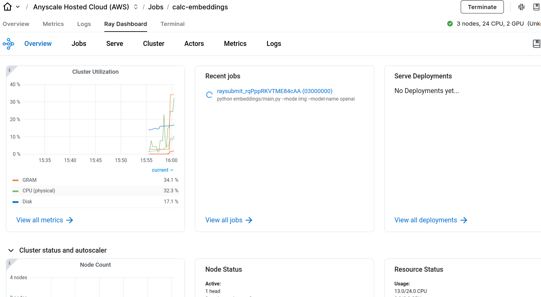Fig. 5 View of the Anyscale Console for Jobs where you can monitor, e.g., cluster utilization, running jobs, and resource usage.

Link4. Application architecture

The application comprises several components that communicate with each other to perform the calculation of embeddings, cross-modal search, reranking, and finally, visualization of the results. Each part is a standalone Ray Serve Deployment, which facilitates serving, scaling, and introducing batching to each component out of the box.

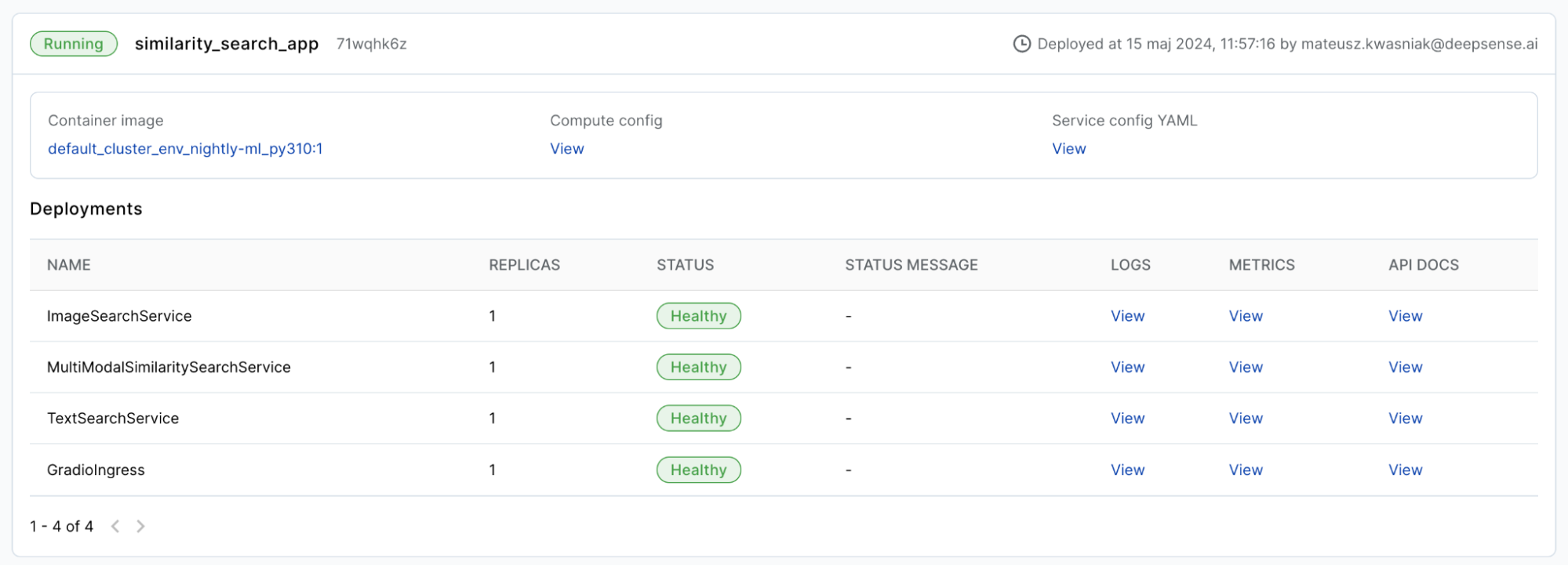Fig. 6 Deployment of similarity_search_app within Anyscale Services (Image by authors).

Anyscale Services allows you to deploy, maintain, and scale Ray Serve applications with ease. It also supports many crucial features such as autoscaling (including scaling to zero replicas), out-of-the-box monitoring of cluster health and services, or rolling deployment strategy.

In addition, it is possible to organize many deployments into a single Ray Serve application, which is a viable option given the deployments can still independently scale but will benefit from being managed and deployed within the same cluster. This is exactly the approach we took while deploying the Similarity Search Application (see Fig. 6). Now, let’s delve deeper into the architecture and its components to explain their purpose and how they communicate with each other.

Fig. 7 Components of the Similarity Search Application (Image by authors).

The system consists of the following pieces:

1. GradioIngress

This is the frontend service that users interact with. It is a set of web UI components designed to make the search easy and intuitive, allowing for simple customization (e.g., model choice, number of results). This is the default entry point to the whole search system, allowing users to only use nice buttons and UI controls without having to worry about any internal logic.

2. Multimodal Similarity Search Service

Under the hood, GradioIngress communicates with the main backend API, which is the Multimodal Similarity Search Service. This component accepts requests for text-based or image-based search, and while in our setup it is solely called by frontend logic, one could interact with the raw backend API as well if necessary (or if we would like to add support for, e.g., a mobile platform).

3. Image Search Service and Text Search Service

Because searching with text is a bit different than searching by image, the core functionality has been delegated to separate services, namely Image Search Service and Text Search Service, which are distinct components within our Similarity Search Application.

Thanks to this, both services can be scaled independently based on traffic (see Figure 8) and maintain their own replicas. Ray Serve's autoscaling can be configured to set minimum/maximum number of replicas and also to set a desired traffic profile per replica by setting target_ongoing_requests.

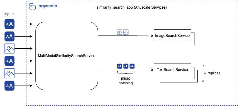Fig. 8. We introduced autoscaling and batching to increase application performance (Image by authors).

These two services know how to transform the input query (text or image) into embeddings using a model chosen by the user (OpenAI or FashionCLIP). All files related to the models, i.e. their configuration, tokenizers, and weights, are downloaded from the HuggingFace Hub at the service's startup (which was not an issue because of the small size of the models).

4. Pinecone

As already mentioned, we used the Pinecone database to store both image and text embeddings. Regardless of input modality (text or image), we query both indices in the database to perform a cross-modal search. Then, the obtained results are deduplicated and reranked - more on that in the following section.

Link4.1 Retrieving results 

Services that perform the search take the user’s input and generate appropriate embeddings using general-use or fine-tuned CLIP, depending on the user’s choice. Then, in the Pinecone index, we search for the most similar vectors (embeddings) to the one obtained from the input query. The score is based on cosine similarity.

Fig 9. The schema of the process of obtaining the end results.

Link4.2 Reranking results 

Another key feature of our application is reranking the results. While the user chooses to use either image or text as an input query, our application takes advantage of multi-modality and considers both text-based and image-based embeddings while performing the search.

1def rerank_results(self, results: List[Dict[str, Any]]):
2        all_modalities_unique = []
3        paths_seen = set()
4        for image_info in results:
5            path = image_info["path"]
6            if path not in paths_seen:
7                all_modalities_unique.append(image_info)
8                paths_seen.add(path)
9        sorted_results = sorted(
10            all_modalities_unique, key=lambda x: x["score"], reverse=True
11        )
12        return sorted_results

This is why, after retrieval of the embeddings from both modalities, we need to aggregate the results. We use a simple reranking mechanism that selects the top K (most similar) results regardless of their modality. We also ensure that the final K results (where K is the number of results to be shown, requested by the user) are unique, i.e., do not contain duplicates, which may occur when we query multiple modalities.

Link5. Using fine-tuned vs. original CLIP

Incorporating two models for embedding generation was a great opportunity to showcase their differences. We visualized the outputs of the OpenAI CLIP model and FashionCLIP on longer and more complex prompts. In our experiment, we used descriptions generated by GPT-3.5 with the prompt “Give me a list of sophisticated outfit descriptions, focus on colors and style of the clothing”, and we searched in the image space (image embeddings). To match the text and image, we took the pair (image, description) with the highest cosine similarity value.

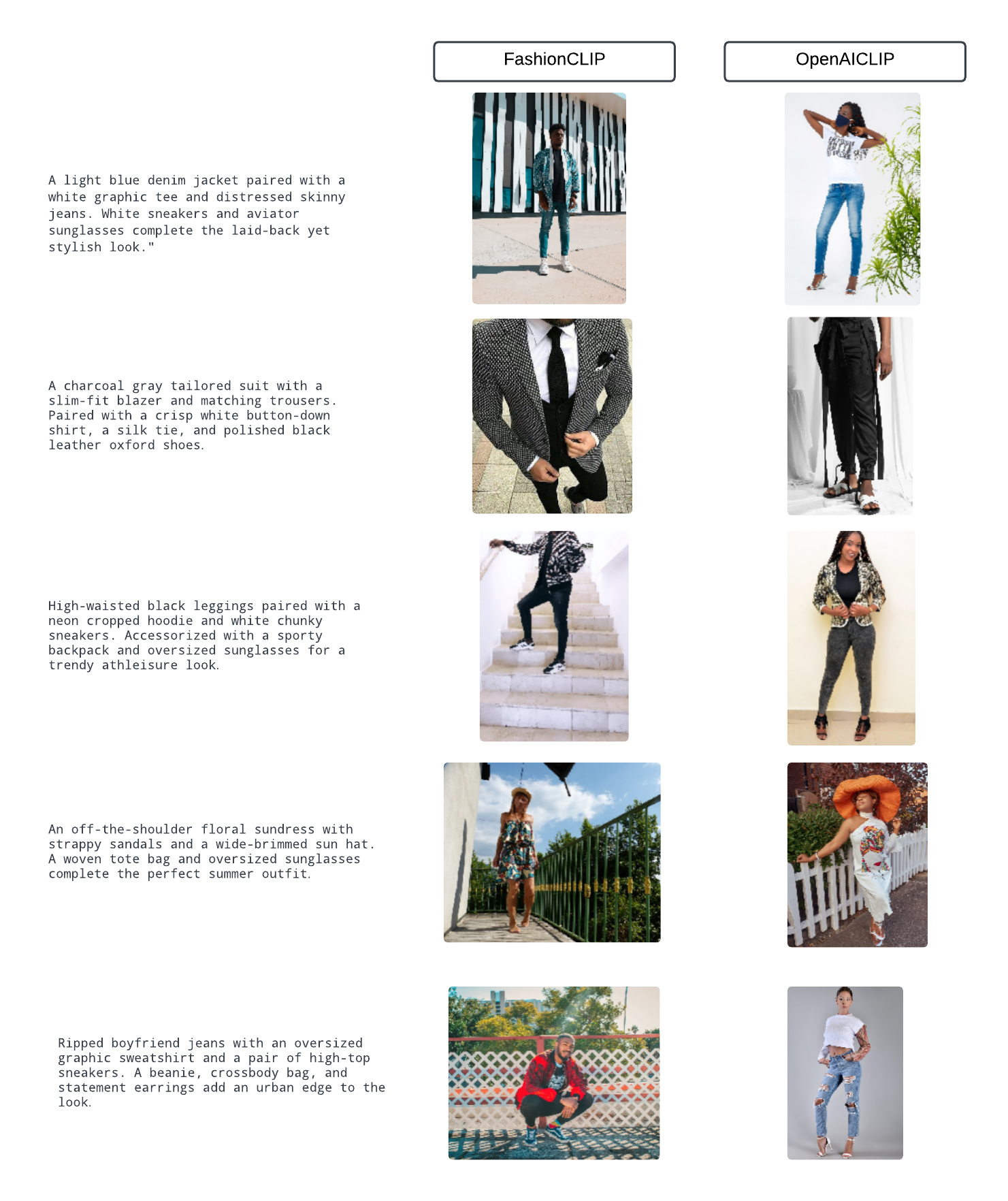Fig. 10 A comparison of the outputs of the text2image retrieval experiment with FashionCLIP vs OpenAI CLIP. Image descriptions obtained by ChatGPT, images from InFashAIv1 dataset.

It appears that OpenAI CLIP tends to focus more on specific parts of clothing, for example, a sun hat or ripped jeans. FashionCLIP performs better in terms of understanding the vibe of an outfit (e.g., “laid-back”), and it seems to consider the attire as a whole. Unfortunately, FashionCLIP sometimes ignores the absence of elements (glasses, hat, etc.) or does not focus on every item's aesthetic (in the first example: the white graphic tee). Using both models in tandem can provide comprehensive results, benefiting from OpenAI CLIP's attention to specific clothing items and FashionCLIP's holistic understanding of an outfit’s vibes.

Link6. Conclusion

In conclusion, this blog post is a comprehensive guide to constructing a fashion image retrieval application from scratch. Through our collaborative efforts, deepsense.ai and Anyscale provided a practical roadmap for building efficient, scalable, and intuitive applications.

Specifically, we've:

• Showcased the efficiency of parallelization techniques offered by Ray Data.

• Demonstrated the creation of Pinecone indexes - where image and text embeddings are stored.

• Leveraged CLIP models to build a cross-modal retrieval pipeline.

• Optimized application performance, exhibiting the directness of using Ray Serve for autoscaling.

• Developed an intuitive Gradio interface that’s easy to modify and extend.

 We've carefully outlined each step, empowering developers to replicate our work.

You can find full implementation on GitHub: cross modal search for ecommerce.

Link7. Future work

In future work, we aim to explore recent multi-modal models like LLaVA and PaliGemma, as they offer exciting possibilities for improving retail and e-commerce systems. From personalized recommendations to providing product insight and assisting in answering product-related queries, multi-modality can improve the customer experience. Benchmarking these architectures focusing on the speed and quality of responses in retail-related tasks will provide valuable knowledge for AI engineers developing similar applications.