Multi-model composition with Ray Serve deployment graphs

Machine learning serving pipelines are getting longer, wider, and more dynamic. They often consist of many models to make a single prediction. To support complex workloads that require composing many different models together, machine learning applications in production typically follow patterns such as model chaining, fanout and ensemble, or dynamic selection and dispatch.

Figure 1: Chaining multiple models in sequence. This is common in applications like image processing, where each image is passed through a series of transformations.

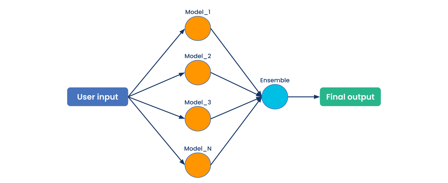Figure 2: Ensembling multiple models. Often, business logic is used to select the best output or filter the outputs for a given request.

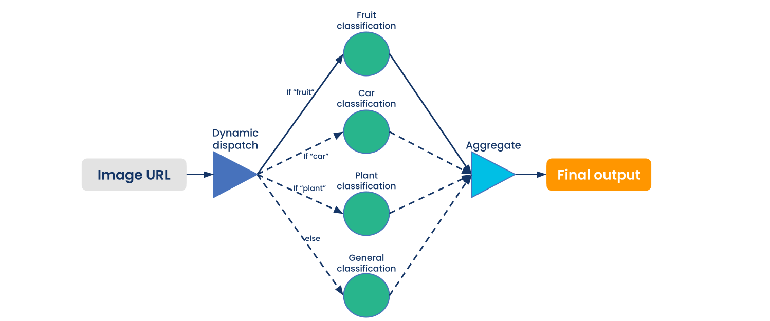Figure 3: Dynamically selecting and dispatching to models. Many use cases don’t require every available model for every input request. This pattern allows only querying the necessary models.

Ray Serve was built to support these patterns and is both easy to develop and production ready. But after listening to Ray Serve users, we've identified ways to improve the process of composing and orchestrating complicated deployment graphs.

Say hello to the Ray Serve Deployment Graph API, now in alpha, which allows developers to build scalable and flexible inference serving pipelines as directed acyclic graphs (DAGs) that take advantage of Ray's compute for scaling.

In this blog post, we'll explain how the Deployment Graph API enables fast local development to production deployment and is scalable with a unified DAG API across Ray libraries. We'll also walk through a real-world example of how to build, iterate, and deploy a deployment graph with the API.

LinkStrengths of Ray Serve

Ray Serve has unique strengths suited to multi-step, multi-model inference pipelines: flexible scheduling, efficient communication, fractional resource allocation, and shared memory. The Deployment Graph API enables users to develop complex machine learning pipelines locally and then deploy them to production with dynamic scaling and lightweight updates (e.g., for model weights).

Compared to other serving frameworks' inference graphs APIs, which are less pythonic and in which authoring is dominated by hand-writing YAML, Ray Serve offers easy, composable, and pythonic APIs, adhering to Ray's philosophy of simple API abstractions.

LinkDeploying a single model

With our current @serve.deployment decorator, users can easily add the decorator to a class or function to make it a serve Deployment, and get two exposed channels to invoke it either via HTTP with FastAPI integration, or Python deployment handle.

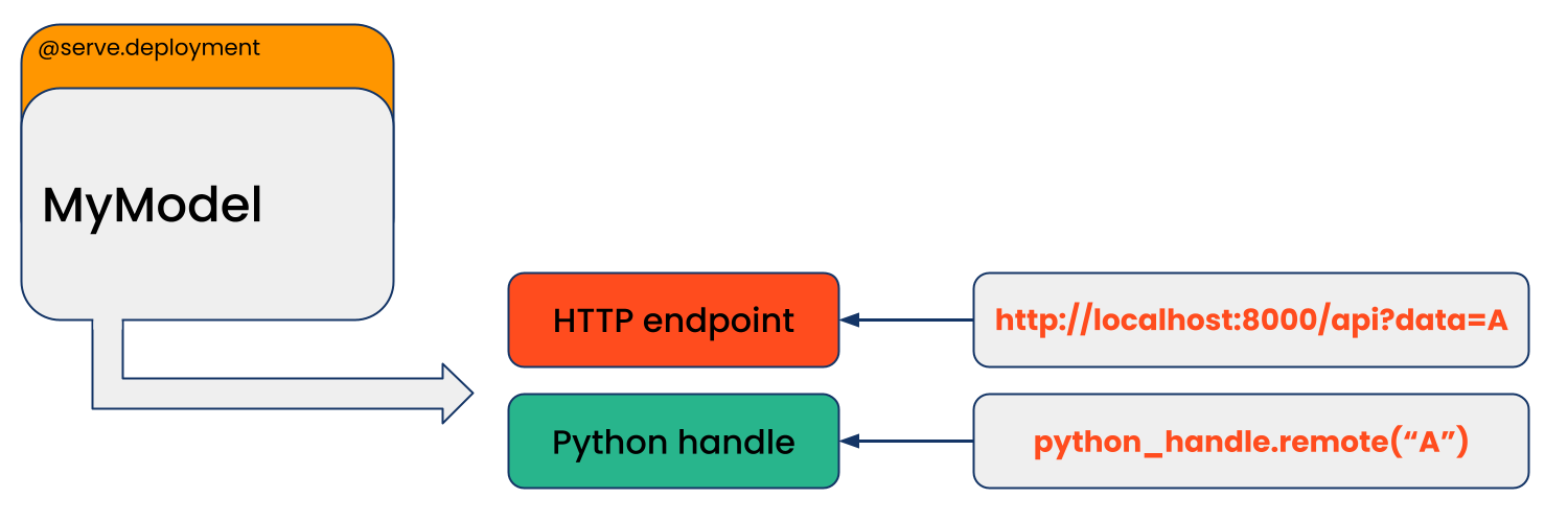Figure 4: Serve Deployment API for single deployment

The Python deployment handle is what people primarily use to compose and orchestrate complicated deployment graphs. While this deployment decorator can take a single Python function or class and convert it into a singular model deployment, there could be business use cases where multiple models and many steps produce the final inference. One solution is to use Python handles to build the inference graph dynamically, which we will explore next.

LinkBuilding a complex deployment graph based on Python handle 

After collecting feedback from existing Ray Serve users, we found that composing graph DAGs with the existing Python handle could be improved. For example, consider the following diagram that shows a content understanding pipeline with graph structure and implementation presented side by side.

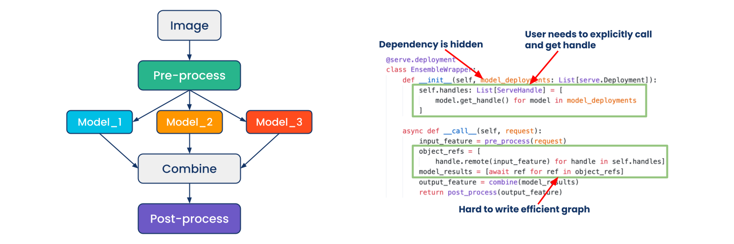Figure 5: Content understanding pipeline with deployment handle

On the left, reading from top to bottom: 

1. Send an image to preprocessing node

2. Forward to three downstream models in parallel 

3. Combine outputs of each model

4. Send to final node to do post processing

In the sample code on the right, we define a wrapper deployment that gets deployment handles to a number of other models. Then when a request comes in, we use the handles to broadcast and evaluate each of the models. Finally, we have some post processing for the result.

This implementation does what we set out for, but it has some problems that need to be addressed:

The graph structure is hidden in the logic of the entire codebase. This means our users need to read the entire codebase and track down each handle in order to see how the graph is composed, without a static definition of the topology. In order to test the graph, users need to manually write a deployment script that deploys each deployment in the correct topological order

It’s hard to operationalize the deployment graph for production. Given the observation above, it’s also difficult to take some operational actions of the deployment graph without diving into the codebase, such as adjusting parameters like num_replicas, update link to latest model weights, etc.

It can be hard to optimize the graph. If you look carefully at the code snippet above, it called await in a loop as an anti-pattern, since we will wait for each result to return one by one instead of parallelizing them. With a static graph definition, we can avoid these performance bugs and provide advanced support for optimizations such as fusing or co-locating nodes on the same host.

LinkOur solution: Ray Serve Deployment Graph API

We designed and implemented the Deployment Graph API with the following features:

• Python native. Instead of writing a YAML file, we make Python the first-class authoring experience with syntax that aligns with current Ray APIs, where chaining, parallelization, ensemble, and dynamic dispatch patterns can be easily expressed with plain Python code.

• Fast local development to production deployment. We take local development experience seriously and provide APIs to make iteration as pleasant as possible while paving a clear road from local development to large-scale production deployments.

• Independently scalable. We discovered a common pattern where a single node acted as the bottleneck, affecting the entire graph’s latency or throughput, so we ensure each node in the deployment graph is independently scalable by design.

• Unified DAG API across the Ray ecosystem. In Ray 2.0, we will have a unified DAG API that is consistent across Ray Core, Ray Serve, Ray Datasets, and Ray Workflows.

LinkExample: Scalable image processing pipeline for content understanding

For the rest of this blog, we will use Figure 6 below as the reference architecture, and will show you how to build it step-by-step using the Deployment Graph API with the following properties:

• Each “node” in the deployment graph is a Ray Serve deployment where 

  • The deployment consists of multiple tasks or actors in a group.

  • Each task or actor can require fractional CPU or GPU resources.

  • The deployment spans across multiple hosts in the cluster.

  • The deployment is independently scalable and configurable with rolling updates.

• End-to-end graph consists of the patterns we mentioned at the beginning: longer (chaining), wider (parallel fanout with ensemble), and dynamic dispatch. All with simple Python code.

Figure 6: Scalable image processing pipeline for content understanding

Now let’s get to the first step from the user input on the far left, which in this case is an image URL, to a deployment that is dedicated to downloading images.

LinkStep 1: User input to downloader node

The code we need to construct a simple user input to downloader connection as shown in Figure 7 below is simple:

Figure 7: Step 1 - Add user input to downloader

1
2
3
4
5
6
7
8
9
10
11
12
@serve.deployment
class Downloader:
   ...
   def run(self):
       pass

# Create a downloader node by binding on its constructor
downloader = Downloader.bind() 

with InputNode() as image_url:
   # Bind image_url to class method "run" of downloader node
   dag = downloader.run.bind(image_url)

The InputNode is a special node in the graph that represents the user input for the graph, which will be resolved to a Python object value at runtime. 

.bind() is our graph building API that can be called on a decorated function, class, or class method. Its syntax is very similar to Ray’s .remote() except upon each call it creates a node that acts as the building block of the DAG.

In this step, we’re using .bind() to send the user input value created by InputNode() to the downloader node.

Note that at deployment graph authoring time, we only need to instantiate and bind the Downloader as if it’s a regular Python class, and use its class method. The user will automatically get what a Ray Serve deployment offers, such as scaling and fine-grained fractional resource allocation with custom configs, as shown in the diagram.

LinkStep 2: Extending the chain 

Next, let’s continue building the chain by connecting the preprocessor node with previous components. For simplicity, we will skip the class definition of Processor — let’s say it has a class method called “process”.

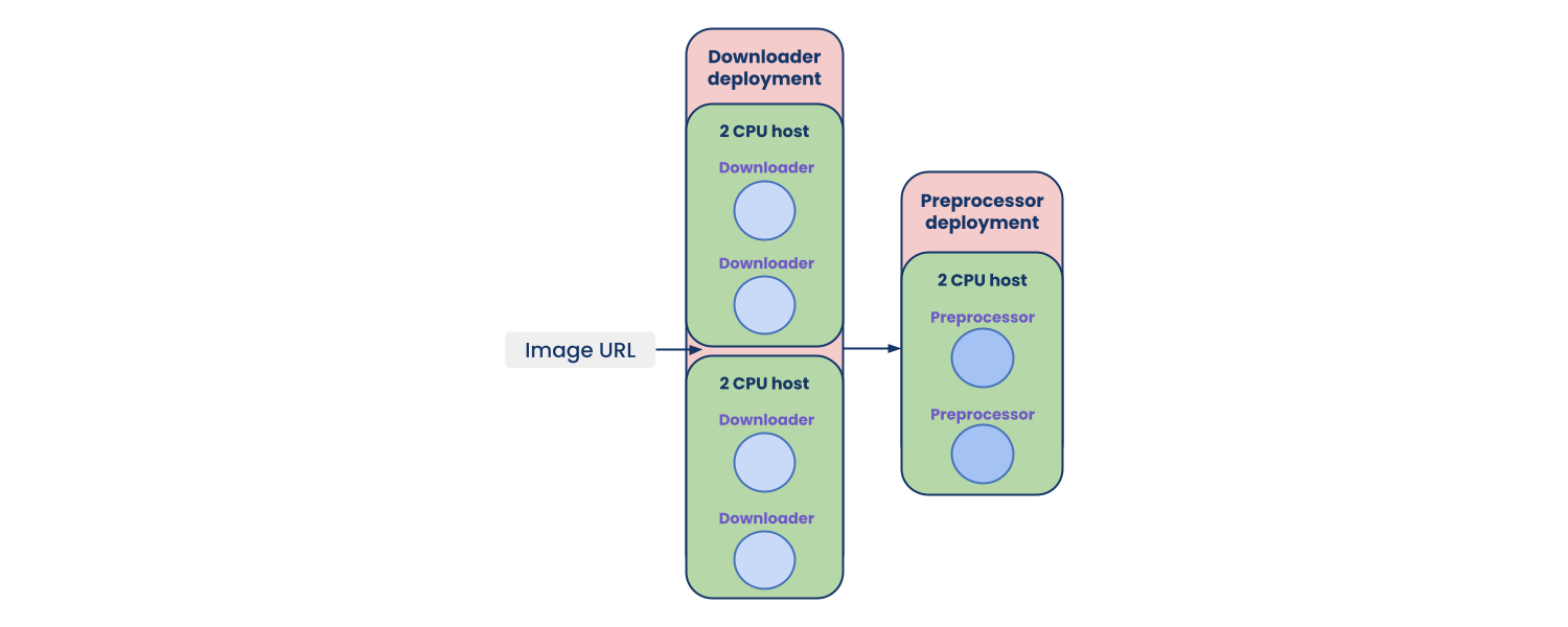Figure 8: Step 2 - Send downloaded image to preprocessor

1
2
3
4
5
6
7
8
9
10
# Create a downloader node by binding on its constructor
downloader = Downloader.bind()
# Create a preprocessor node by binding on its constructor
preprocessor = Preprocessor.bind()

with InputNode() as image_url:
   # Bind image_url to class method "run" of downloader node
   downloaded_image = downloader.run.bind(image_url)
   # Bind intermediate downloaded image to preprocessors' class method
   dag = preprocessor.process.bind(downloaded_image)

We can see extending a new node in the chain is as simple as binding a new instance, and passing the previous step’s output downloaded_image variable to the processor’s class method process. The value of downloaded_image will be resolved to a Python object at runtime, and fed as input to process.

LinkStep 3: Add parallel calls 

Now that we have the processed image, let’s proceed with sending it to two separate downstream nodes in parallel. Note that they can be co-located on the same host where each of them can take fractional GPU, which is supported natively by Ray Serve.

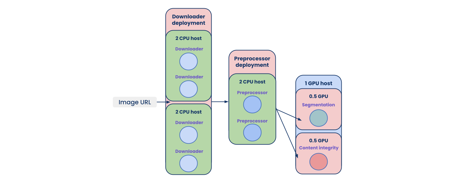Figure 9: Step 3 - Send image to downstream models in parallel

1
2
3
4
5
6
7
8
9
10
11
12
13
14
15
16
# Create a downloader node by binding on its constructor
downloader = Downloader.bind()
# Create a preprocessor node by binding on its constructor
preprocessor = Preprocessor.bind()

segmentation_model = Segmentation.bind(weights="s3://bucket/file")
integrity_model = Integrity.bind(weights="s3://bucket/file")

with InputNode() as image_url:
   # Bind image_url to class method "run" of downloader node
   downloaded_image = downloader.run.bind(image_url)
   # Bind intermediate downloaded image to preprocessors' class method
   processed_image = preprocessor.process.bind(downloaded_image)

   segmentation_output = segmentation_model.forward.bind(processed_image)
   integrity_model = integrity_model.forward.bind(processed_image)

Expressing parallel calls is very trivial: just use the same variable. The same variable name (backed by an IR node behind the scene) will be resolved to the same value in separate nodes.

LinkStep 4: Add dynamic dispatch 

Now let’s add another edge to the graph where dynamic dispatch happens. It will receive the same image as two other nodes, but at runtime it will dynamically choose only one path, depending on the metadata of the image based on its category.

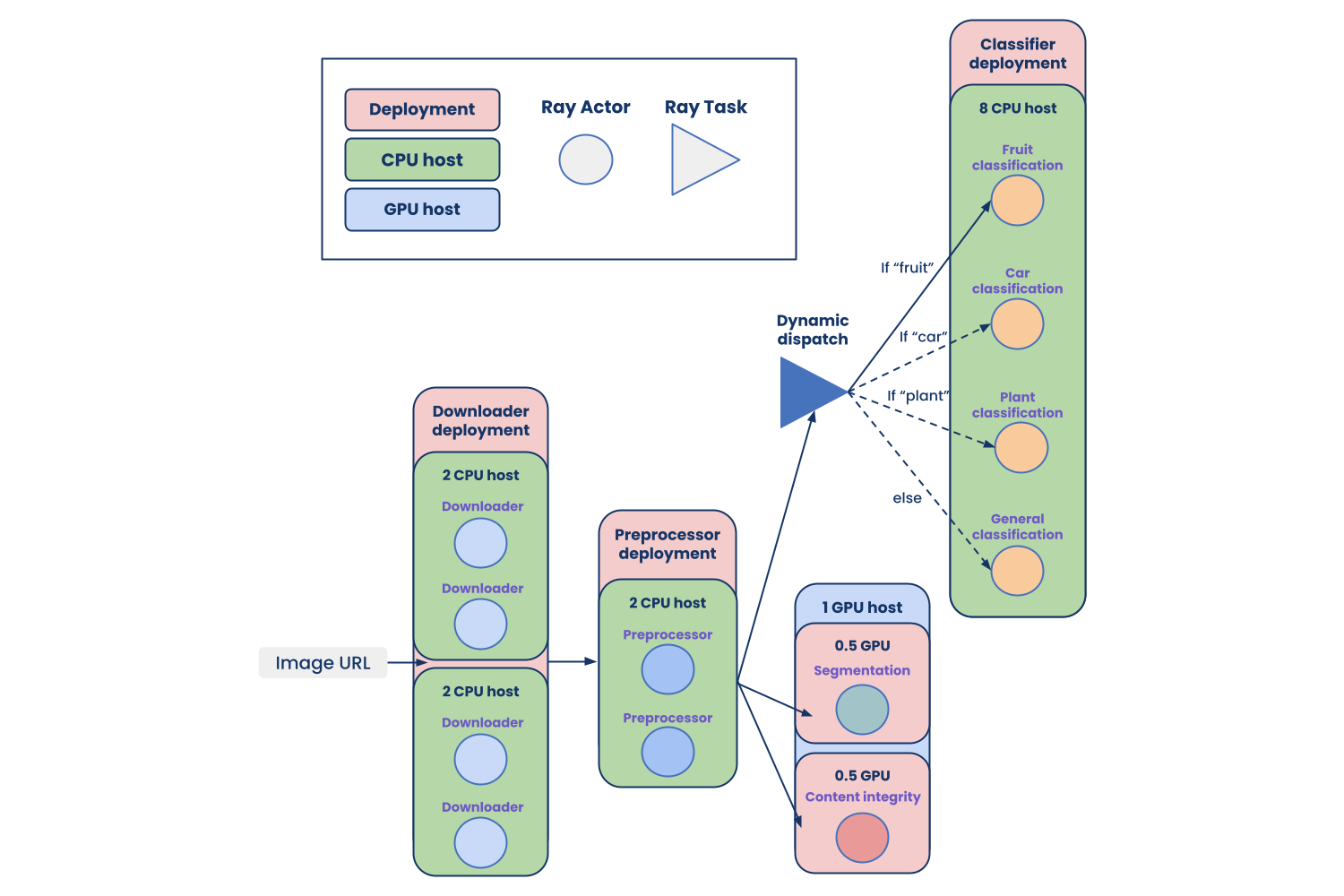Figure 10: Step 4 - Add dynamic dispatch

1
2
3
4
5
6
7
8
9
10
11
12
13
14
15
16
17
18
19
20
21
22
23
24
25
26
27
28
29
30
31
32
33
34
35
36
@serve.deployment
class Dispatcher:
   def __init__(self, fruit_model, car_model, plant_model, general_model):
       # Upstream nodes can be passed into constructor and used in class
       # method calls
       self.fruit_model = fruit_model
       self.car_model = car_model
       self.plant_model = plant_model
       self.general_model = general_model

   async def run(self, image, metadata):
       # Dynamic dispatch can be simply expressed in python with Ray API calls
       if metadata == "fruit":
           return await self.fruit_model.remote(image)
       elif metadata == "car":
           return await self.car_model.remote(image)
       elif metadata == "plant":
           return await self.plant_model.remote(image)
       else:
           return await self.general_model.remote(image)

fruit_model = Fruit_Classification.bind(weights="s3://bucket/file")
car_model = Car_Classification.bind(weights="s3://bucket/file")
plant_model = Plant_Classification.bind(weights="s3://bucket/file")
general_model = General_Classification.bind(weights="s3://bucket/file")
dispatcher = Dispatcher.bind(fruit_model, car_model, plant_model, general_model)

with InputNode() as image_url:
   # Bind image_url to class method "run" of downloader node
   downloaded_image = downloader.run.bind(image_url)
   # Bind intermediate downloaded image to preprocessors' class method
   processed_image = preprocessor.process.bind(downloaded_image)

   ...

   dag = dispatcher.run.bind(processed_image, "plant")

Creating individual model nodes is the same as previous steps. There are a few new pieces regarding building dynamic dispatch that illustrate some properties of our API:

• Nodes can be passed into another node’s constructor and assigned as an instance variable. 

• At runtime, control flow and dynamic dispatch can be easily expressed with plain Python code.

LinkStep 5: Add ensemble aggregator

Now we’re at our last step of combining outputs from multiple nodes in an aggregator. We can easily express this as a plain function node in the graph:

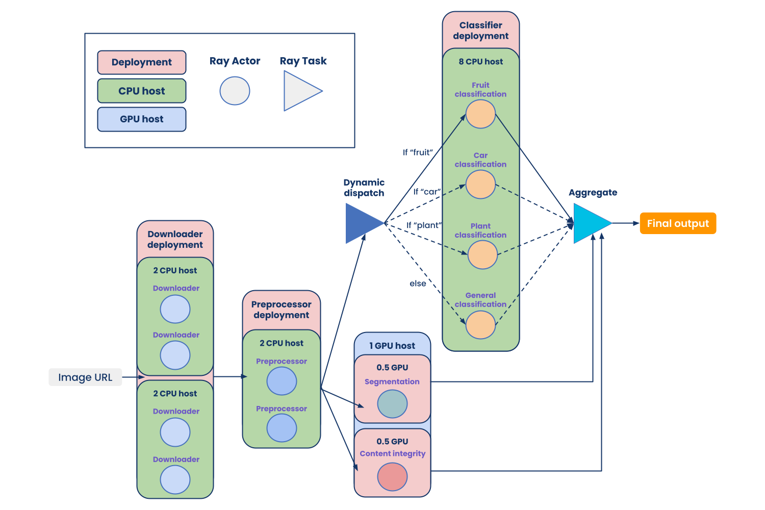Figure 11: Step 5 - Add ensemble

1
2
3
4
5
6
7
8
9
10
11
12
13
14
15
16
17
@serve.deployment
def aggregate_fn(segmentation_output, integrity_output, dispatched_output):
   return segmentation_output + integrity_output + dispatched_output

with InputNode() as image_url:
   # Bind image_url to class method "run" of downloader node
   downloaded_image = downloader.run.bind(image_url)
   # Bind intermediate downloaded image to preprocessors' class method
   processed_image = preprocessor.process.bind(downloaded_image)

   segmentation_output = segmentation_model.forward.bind(processed_image)
   integrity_output = integrity_model.forward.bind(processed_image)
   dispatched_output = dispatcher.run.bind(processed_image, "plant")

   dag = aggregate_fn.bind(
       segmentation_output, integrity_output, dispatched_output
   )

At this step you can see more attributes of the Deployment Graph API:

• A function can be used as a node in a graph. 

• We can pass values as well as other nodes as input to the function node.

LinkStep 6: Defining HTTP input

At this stage we’ve built the body of the DAG with Python APIs that facilitate local execution with Ray. The next step is to configure the serving aspect, such as HTTP endpoint, HTTP input adapter, and Python handle.

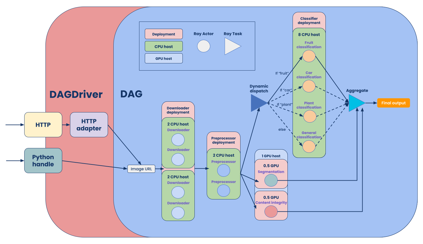Figure 12: Step 6 - Add DAGDriver deployment for HTTP

1
2
3
4
5
6
7
8
9
10
11
12
13
from ray.serve.drivers import DAGDriver
from ray.serve.http_adapters import json_request

with InputNode() as image_url:
   ...

   dag = aggregate_fn.bind(
       segmentation_output, integrity_output, dispatched_output
   )

   serve_dag = DAGDriver  \
       .options(num_replicas=3, route_prefix="/my_graph")  \
       .bind(dag, http_adapter=json_request)

There are two new concepts for this:

DAGDriver: The ingress component of your deployment graph that holds the graph as a DAG Python object. It’s a regular Ray Serve deployment object that can be configured and scaled independently. 

http_adapter: Facilitates conversion of HTTP raw input into a Python object schema.

DAG Driver is a regular Ray Serve deployment that can be independently scaled and configured with custom HTTP options. It exposes the same entries like current deployment: HTTP and Python handle, with a few built-in components to facilitate HTTP request -> Python object adaption. You can learn more about it in our documentation.

Also check out our working demo of building a content understanding graph using our API.

LinkStep 7: Running the deployment graph

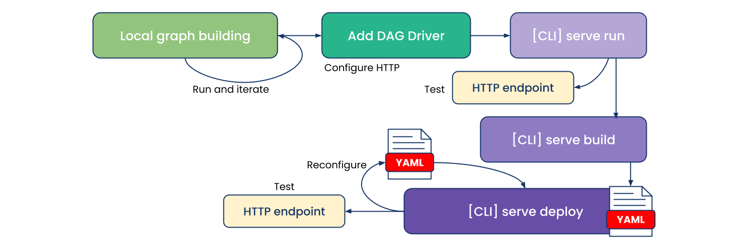Figure 13: Step 7 - Deployment Graph iteration and deployment cycle

This flow chart shows our designed local development and production deployment flow of a deployment graph, from the Python incremental build to iteration of the body of your DAG to adding Ray Serve attributes such as HTTP endpoint and adapter.

The green blocks and serve run in Figure 13 are available in Ray 1.12.1, and the purple blocks such as serve build and serve deploy are in active development.

You might notice we only covered the green blocks in the diagram from the authoring and development side. We have more work in progress that further enhances the operational aspects of deployment graphs such as REST API/CLI to build your deployment graph into YAML files to facilitate declarative and idempotent operations. Stay tuned for future blog posts!

LinkFuture improvements 

We plan to continue to improve the Deployment Graph API in future releases. Current items on our roadmap include:

• Operationalizing deployment graphs to pave the way from local development to remote clusters in production

• Performance optimizations based on given static graph topology

• ModelMesh layer on Ray

• Model multiplexing on the same host

• Scale-to-zero with lazily invoked models

• Better UX and visualization support

LinkBonus: Unified Ray DAG API

DAG is a very common abstraction that we see across many computation tasks. In our design of the DAG API, we put in a lot of effort to ensure it has the right layering under one set of unified APIs for authoring and execution, but also exposes the right abstractions for library-specific executor and options.

You can learn more about this in our Ray 2.0 design doc.

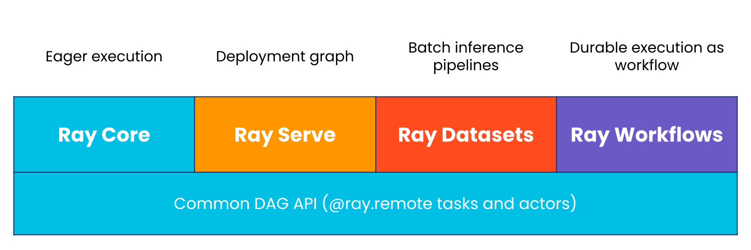Figure 14: Unified Ray DAG API

LinkConclusion 

We’ve reviewed how our users currently use deployment handles to compose complex deployment graphs and challenges we’ve observed for this increasingly important workload: no static graph definition, which leads to challenges of operationalizing deployment graphs without codebase context, and the missed opportunity to optimize performance of deployment graphs.

We then showed how the new Deployment Graph API in Ray Serve addresses these challenges and walked through a real-world example of how to build, iterate, and deploy a deployment graph with the API. The Ray Serve Deployment Graph API is Python-native, enables fast local development to production deployment, and is scalable with a unified DAG API across Ray libraries.

We value input from the Ray community!  If you’re ready to get started with Ray Serve or the Deployment Graph API, check out the detailed tutorial in our documentation. If you have suggestions on how the Deployment Graph API can work better for your use case, head over to our user forums or file an issue or feature request on GitHub. We can’t wait to partner with you to adopt Ray Serve in your project. Let’s get in touch as well!

If you’re interested in our mission to simplify distributed computing, we’re actively hiring across the company.

LinkResources

• Ray Meetup: Productionizing ML at scale with Ray Serve

• Ray docs: Deployment Graph 

• Ray docs: HTTP adapters