We're pleased to announce significant improvements to Ray Data over the last few releases, including features such as:

• Native join support via the ds.join() API

• Key-based repartitioning with repartition(key=...)

• A new, simpler custom aggregation API with AggregateFnV2

• Improved performance of large scale sorting, which improves range partitioning shuffle 

One particular feature we want to highlight in the most recent Ray 2.46 release is a new hash-based shuffle backend that powers

• Joins

• Better performance for repartitioning (as well as repartitioning by key)

• Better performance for aggregations.

On top of significant runtime improvements for repartitioning and aggregations, it also dramatically reduces memory pressure compared to previous shuffle implementation.

Below, we discuss how this new backend works and discuss benchmarks highlighting its improved performance on key Ray Data workloads. 

LinkWhy Hash Shuffle?

LinkPrior approach: Range-Based Shuffle

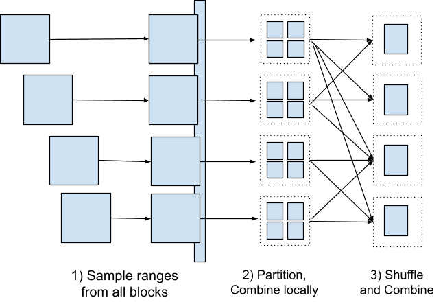
In previous versions of Ray Data, shuffling relied on a range-partitioning approach. In this approach:

• First, we collect samples from every block and used to determine approximate range boundaries (based on the target number of partitions)

• Every input data block is split into N partitions based on determined boundaries

• Individual partitions are shuffled and then combined with other partitions w/in the same range clumped together.

This approach has several obvious limitations: 

• The number of objects created in this approach is O(N * M), where N is the number of incoming blocks and M is the target number of resulting partitions (by default M = N). For example, if your input dataset has 1000 blocks and 1000 resulting partitions, then you’d be producing 1M range-partitions in the process. All of this was coordinated by a single driver process on the Ray cluster head node and was easily bottlenecked at scale.

• The prior implementation of the shuffle also deferred the range-sampling operation until all blocks become available, keeping the pipeline idle for prolonged period of time and increasing peak memory usage.

LinkIntroducing Hash-Based Shuffle

The new hash shuffle implementation offers an alternative, simpler and more efficient approach which tackles the above issues. 

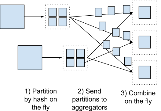
• Every arriving block is hash-partitioned based on the tuple of its key-values (values in key columns for joins/repartition/groupby operations)

  • We hash-partition by computing hash(key_tuple) % num_partitions for every row, splitting the block into partition-shards.

• The shards are then sent to a corresponding Aggregator actor (for specific partition). 

• Aggregator actor then subsequently combines these shards into the new partition, additionally executing downstream operators (like join, aggregations) or simply output the partition in case of repartitioning.

This design allows us to start “shuffling” part of the operation immediately as soon as the first input blocks arrive instead of deferring it until the whole dataset is materialized.

LinkImplementing Joins on Hash Shuffle

In 2.46 Ray Data added support for inner, left/right/full outer joins.

Joins are leveraging a new hash-shuffle backend to colocate records with the same keys on the same Aggregator.

1import ray
2
3users_file = "s3://air-example-data/movielens-25m/clean_featurized_data/users.parquet"
4ratings_file = "s3://air-example-data/movielens-25m/clean_featurized_data/ratings.parquet"
5movies_file = "s3://air-example-data/movielens-25m/clean_featurized_data/movies.parquet"
6
7users = ray.data.read_parquet(users_file)
8users = users.drop_columns(["rating_avg", "rating_count"])
9movies = ray.data.read_parquet(movies_file)
10ratings = ray.data.read_parquet(ratings_file)
11
12users_with_ratings = users.join(
13    ratings, num_partitions=20, on=("userId",), join_type="inner")
14all_combined = users_with_ratings.join(
15    movies, num_partitions=20, on=("movieId",), join_type="inner")
16print(all_combined.take(100))

To join localized partitions with the best possible performance we’re staying clear of performing any CPU-intensive operations in Python and instead opting to (currently) leverage Apache Arrows’s Acero engine by utilizing PyArrow’s native Table.join operation. 

It’s worth noting that in our internal testing we observed that Acero join operations are memory-heavy which requires provisioning of substantial heap memory capacity in addition to Ray’s Object Store memory necessary to facilitate blocks transfer b/w the nodes. In the near future we’ll be evaluating alternatives to perform joins as efficiently as possible.

LinkPerformance Benchmarks

Our benchmarks reveal substantial improvements across various workloads. Tests were conducted on a cluster with 1 m7i.4xlarge (16 CPU / 64 GB) and 5 m7i.16xlarge (64 CPU / 256 GB). Object store memory on each worker node was set to 128GB, and num_cpus on the head node was set to 0.

We run 3 workloads:

• Preprocessing workload: This workload consists of a chain of imputation and normalization operators (via the SimpleImputer and StandardScaler preprocessors), operating on 4 columns from a TPC-H Orders dataset (SF1000).

• TPC-H Q1 SF100: An aggregation-heavy workload from the TPC-H benchmark with several hundreds of millions of elements

• TPC-H Q1 SF1000: An aggregation-heavy workload from the TPC-H benchmark with several billion elements, 

In the below table, we measure the runtime improvement between the range-partitioning shuffle and hash-partitioning shuffle backend. We see that compared to 2.43, hash-based shuffle performance improvements range from 3.3x to 5.6x, and TPCH-Q1-SF1000, which previously couldn’t complete on the given cluster size, is now feasible.

We also note that on the same workloads, we’ve also improved range-partition shuffling as well. Compared to 2.43, we see that range-partitioning shuffle improves workloads from 1.6x to 4.3x in terms of runtime.

Beyond raw speed, hash shuffles can also reduce memory pressure. Below, we measure the peak memory usage of the workload. In both situations, peak memory usage is reduced significantly by switching to using the hash shuffle backend, with a relative improvement of up to 3.9x.

LinkWhat's Next

Looking ahead, we're excited to build on this foundation with:

• Support for different types of joins

• Support for logical plan optimizations that reorder joins

• Further improvements for Data preprocessors!

You can read more about shuffles and joins on the Ray Data documentation: 

We're eager to see what you build with Ray Data! Join the conversation on Discuss or the #datasets channel in the Ray Slack to share your experiences and suggestions.