Training 175B Parameter Language Models at 1000 GPU scale with Alpa and Ray
This is part 2 of our generative AI blog series. Here we cover how Ray empowers large language models (LLM) frameworks such as Alpa. To learn how to use Ray to productionize generative model workloads, see part 1.
This blog post presents how two open-source frameworks, Alpa and Ray, closely integrate to achieve the scale to train a 175B parameters OPT-175B model (equivalent to GPT-3) with pipeline parallelism up to 1024 A100 GPUs in collaboration with Nvidia. With this integration, our benchmarks show three scaling results:
1. Alpa can scale beyond 1000 GPUs for 175 billion parameter scale LLMs.
2. Alpa can achieve SOTA peak GPU utilization (57.5%) and HW FLOPs per GPU (179 TFLOPs), about 21%~42% higher compared with published LLM benchmarks from Meta, Google, and Nvidia in 2022.
3. All LLM parallelization and partitioning are done automatically with one line decorator.
Alpa and Ray are open source projects that work together to offer a scalable and efficient solution for training large language models at scale. In this blog, we examine how these two integrated frameworks, their combined stack's architecture, developer friendly API, scalability, and performance in detail.
LinkBackground of large language models (LLM)
Because of rapid research in academia and industries, a growing trend in the release of an array of models, with an exponential number of training parameters in billions, ensued in a short span of time, as shown in the figure below. This new wave of machine learning is spearheaded by Generative AI models, including ChatGPT, Diffusion, RoBERTa, DALL-E, which allow users to feed as input into the model different modalities–text, video, audio, and image–to analyze, synthesize, and generate new content as simple sequence-to-sequence tasks. Generative AI is the next era in natural language processing (NLP).
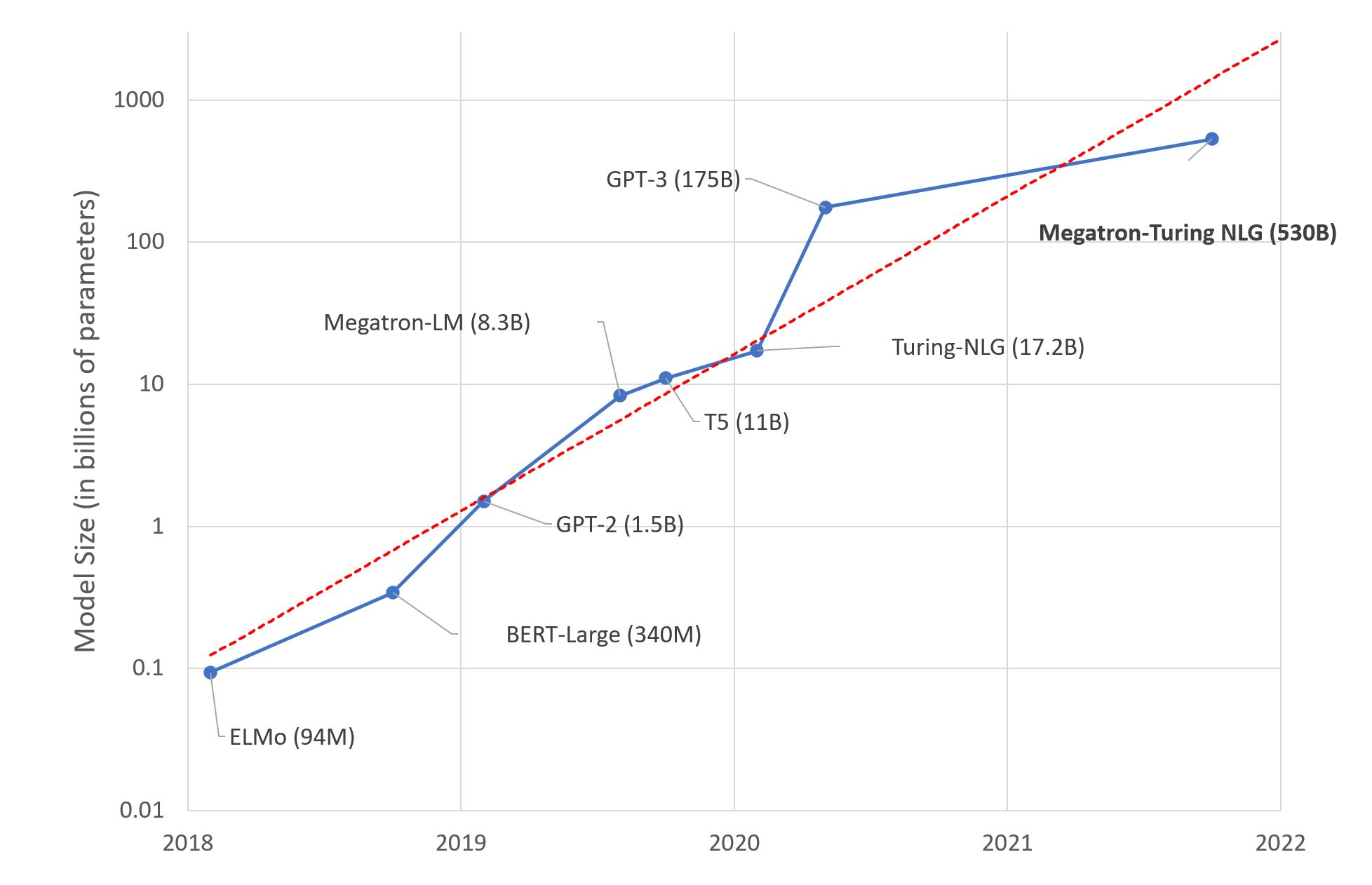 Trend showing LLM models growing in size over the years
But training these LLM models with billions of parameters from scratch or fine tuning with new data has its set of challenges. Training and evaluating demand massive distributed computing power, clusters of accelerated-based hardware and memory, reliable and scalable machine learning frameworks and fault-tolerant systems.
In the next two sections, we discuss some of the challenges, followed by our approach to address them.
LinkMachine learning system challenges of LLM
The parameter size of a modern LLM is at the magnitude of hundreds of billions that exceeds the GPU memory of a single device or host – we call it “the memory wall.” For an OPT-175B model, it requires 350 GB GPU memory to just fit the parameters, not to mention GPU memory needed for gradients and optimizer states during training that can further push memory requirements beyond 1 TB. Meanwhile, commodity GPUs only have 16GB / 24GB GPU memory, even the most advanced A100 and H100 GPUs only have 40GB / 80GB GPU memory per device.
Tools and algorithms such as ZeRO Infinity can help with addressing this “memory wall” problem by allowing you to train much larger models with limited memory, but it often comes at the cost of hardware utilization and efficiency.
In the same spirit of making LLM more accessible, we explored scaling LLM training and inference with all parameters remaining on GPU for best efficiency without sacrificing usability.
In order to efficiently run training and inference for LLMs, we need to partition the model across its computation graph, parameters, and optimizer states such that each partition fits nicely within the memory limit of a single GPU. Based on the GPU cluster available, ML researchers need to devise a strategy to optimize across different parallelization dimensions in order to train efficiently.
Today, however, optimizing training across different parallelization dimensions is manual and difficult. These dimensional partition strategies of an LLM can be categorized as:
Inter-operator parallelism: Partition the full computation graph to disjoint subgraphs. Each device computes its assigned subgraph and communicates with other devices upon finishing.
Intra-operator parallelism: Partition matrices participating in the operator to sub-matrices. Each device computes its assigned submatrices and communicates with other devices when multiplication or addition takes place.
Both strategies can be applied to the same computation graph.
Note: Some research work categorizes model parallelism as “3D-parallelism” that represents data, tensor and pipeline parallelism respectively. In Alpa’s terminology, data is simply the outer dimension of tensor parallelism that maps to intra-operator parallelism, and pipeline parallelism is the result of inter-operator parallelism that partitions graph into separate stages with pipelining orchestration. They are equivalent in power, and we will keep the partitioning terminology simple and consistent to only use inter and intra-op parallelism from here.
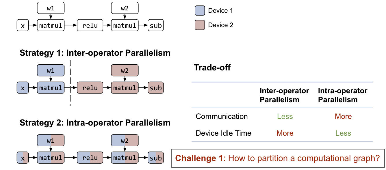 Figure 1: Partition strategies for inter and intra operator of a computation graph
Exploring the possible strategies of inter and intra operator parallelism is a challenging combinatorial problem with tradeoffs. With reasonable computation graph partitioning of inter-operator parallelism, the communication cost can be small between subgraphs but introduces data dependency. Even though pipelining can help alleviate the problem, device idle time is still inevitable.
On the other hand, intra-operator parallelism can parallelize the operator computation among multiple GPU devices with less idle time, but higher communication cost when the next operator cannot preserve matrix partition from the previous one.
In addition to partitioning of matrices and computation graphs, we need the ability to map partitions to GPU devices with awareness of the heterogeneous network topology. GPU connections inside a node (NVLink) are orders of magnitude faster than inter-host networking (InfiniBand, EFA, ethernet), and will lead to significant performance differences among different partition strategies.
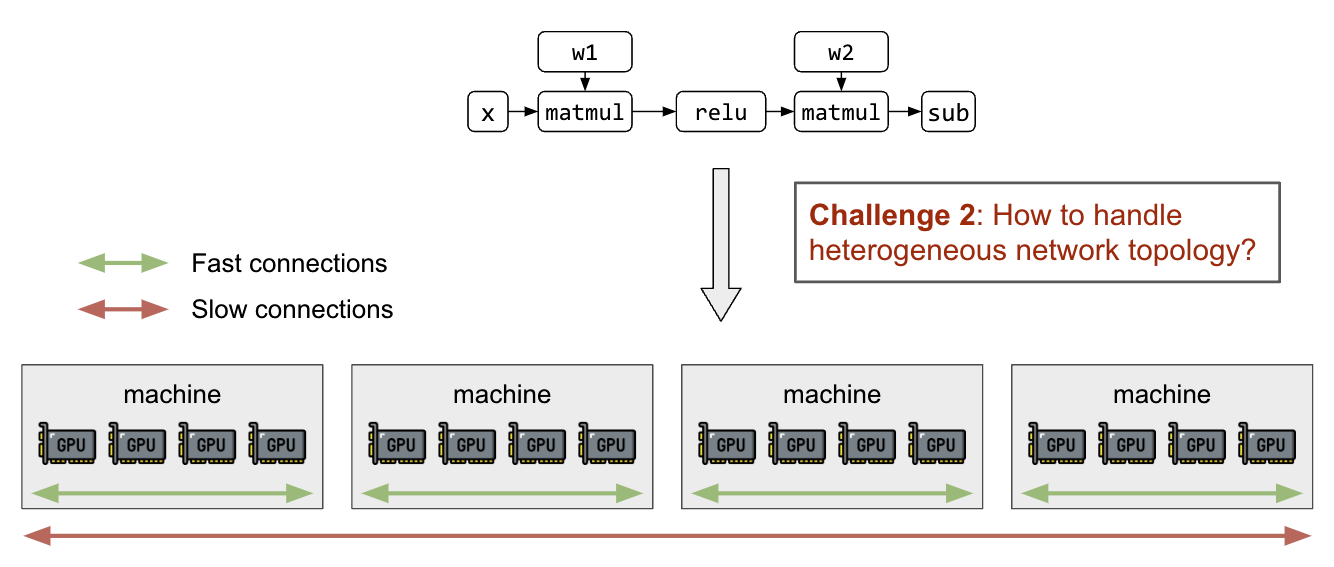 Figure 2: Network topology of GPU clusters
LinkCurrent state of LLM parallelization
There are a number of prior works in the model parallelism domain that achieve different parallelism techniques mentioned above, as shown in the following Figure 3. As illustrated earlier, finding and executing optimal model partitioning strategy is very manual and difficult that requires substantially deep domain expertise.
Alpa handles inter and intra operator parallelism automatically with one line decorator that seamlessly devises a partition strategy for data, tensor and pipeline parallelism for LLM at scale, and is capable of generalizing to a wide range of model architectures that greatly simplifies model parallelism to make LLM more accessible to everyone.
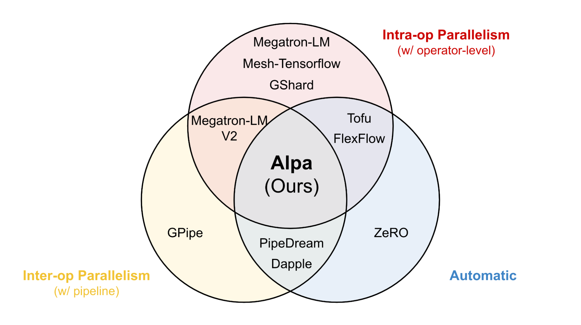 Figure 3: Alpa’s positioning with automatic inter and intra operator parallelism
LinkScalability issues of JAX on GPU clusters
The impact of network topology further manifests into the difference of scaling LLMs for TPU and GPU clusters with their unique hardware level connections.
On a TPU cluster (see Figure 4), the network fabric is specifically designed with a torus topology, so it can scale to thousands of chips with intra-op parallelism only with APIs provided by jax.pjit.
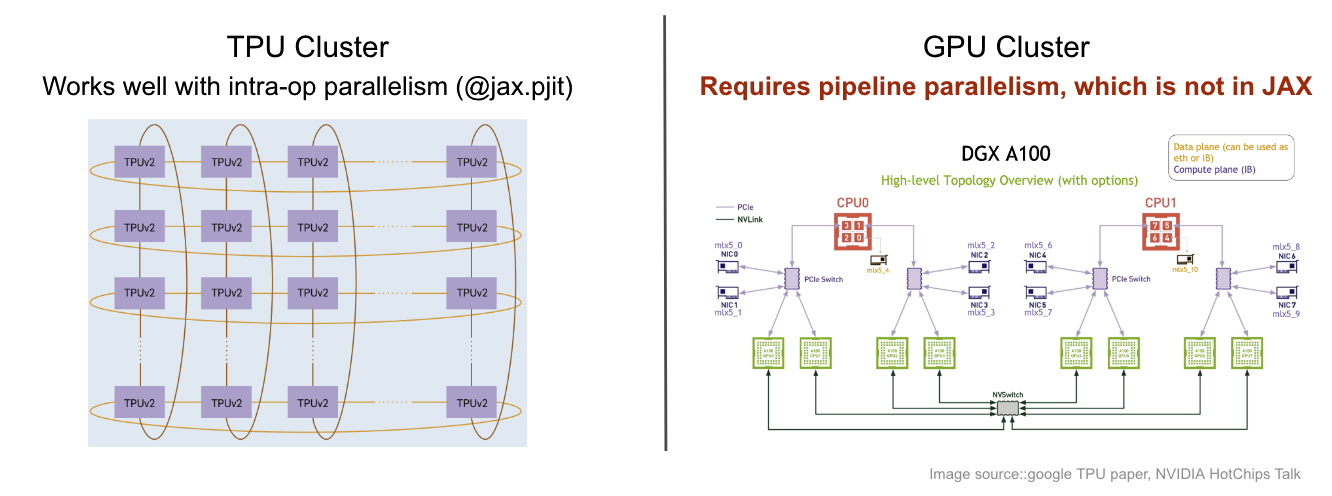 Figure 4: Network topology comparison between TPU and GPU cluster
On a GPU cluster, the network fabric is typically a fat-tree topology with limited inter-host network bandwidth and more challenging to scale up in larger scale clusters, which calls for parallelization plans that are more communication-efficient, such as pipeline parallelism.
However, pipeline parallelism is not provided in JAX currently, thus it limits the scalability of JAX LLM on GPU clusters.
LinkArchitecture overview
Before we dive into how we addressed these challenges with our layered technical stack, it is important to provide an architectural overview of its critical components.
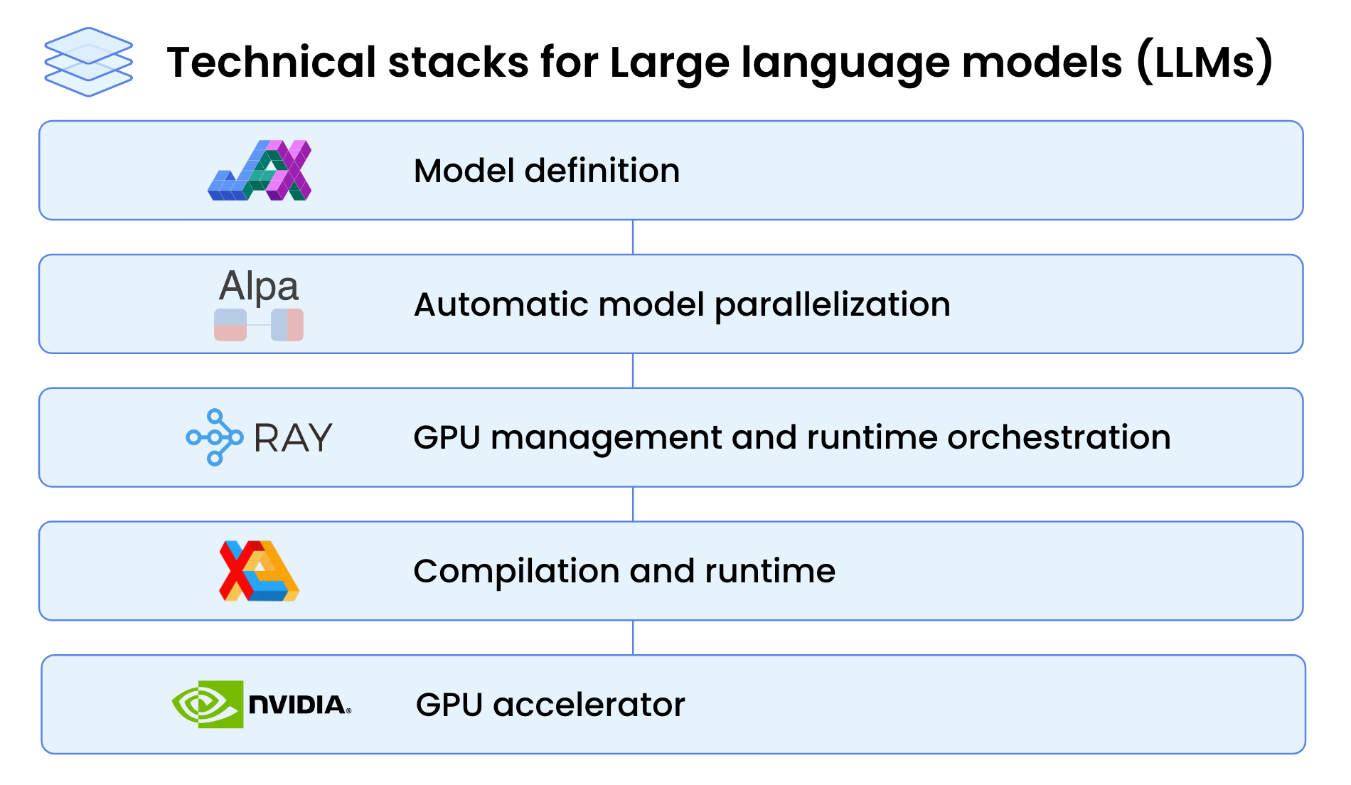 Figure 5: Technical integration layered stack for LLM
LinkIntroduction to Alpa
Alpa is a unified compiler that automatically discovers and executes the best Inter-op and Intra-op parallelism for large deep learning models.
Alpa’s key API is a simple @alpa.parallelize decorator that parallelizes and optimizes for the best model parallelism strategy automatically. Given JAX’s nature of static graph definition with known size and shapes, a simple tracing on the train_step with sample batch is sufficient for us to capture all information we need for automatic partitioning and parallelization. Consider the simple code below.
1@alpa.parallelize
2def train_step(model_state, batch):
3    def loss_func(params):
4        out = model_state.forward(params, batch["x"])
5        return np.mean((out - batch["y"]) ** 2)
6
7    grads = grad(loss_func)(state.params)
8    new_model_state = model_state.apply_gradient(grads)
9    return new_model_state
10
11# A typical JAX training loop
12model_state = create_train_state()
13for batch in data_loader:
14    model_state = train_step(model_state, batch)
15LinkAutomatic parallelization passes in Alpa
Alpa introduces a unique approach to tackle the complex parallel strategy search space of a two-level hierarchical system. Traditional methods have struggled to find a unified algorithm to derive an optimal parallel strategy from the vast space of inter- and intra-operator options. Alpa addresses this challenge by decoupling and reorganizing the search space at different levels.
At the first level, Alpa searches for the most effective inter-operator parallel plan. Then, at the second level, the best intra-operator parallel plan for each stage of the inter-operator parallel plan is derived. This approach works well and the problem is solvable by simplifying the search space with hierarchy and focusing on algorithms optimized for each stage’s cost function for its computational characteristics respectively.
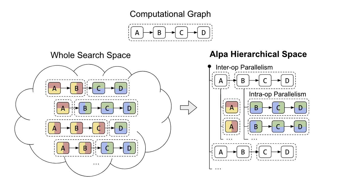 Figure 6: Alpa’s hierarchical search space for partitioning strategy
The Alpa compiler is built around the search space decomposition approach we introduced. Its input consists of a computational graph and a cluster specification. To optimize the parallel strategy, Alpa conducts two compiler passes:
The first pass: inter-operator utilizes dynamic programming to identify the most suitable inter-operator parallelism strategy.
The second pass: intra-operator uses integer linear programming to find the best intra-operator parallelism strategy.
The optimization process is hierarchical, where the higher-level inter-operator pass calls the lower-level intra-operator pass multiple times, making decisions based on the feedback from the intra-operator pass. Finally, the runtime orchestration pass executes the parallel plan and brings the strategy to life.
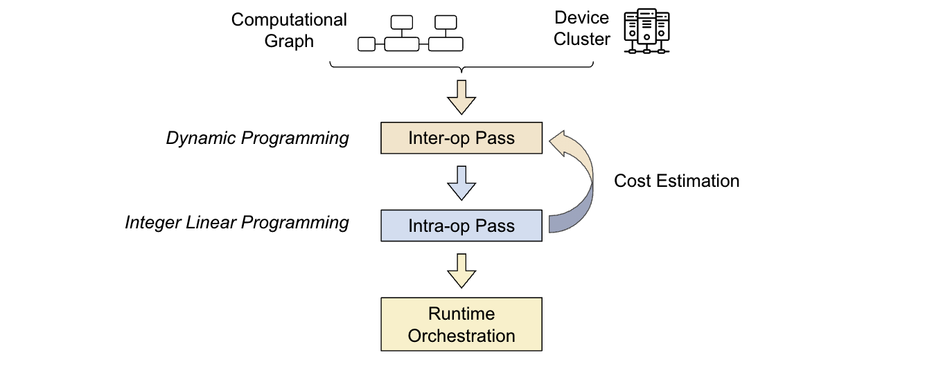 Figure 7: Alpa’s automatic partitioning passes at different levels
In the next section, let’s dive into Ray, a distributed programming framework that Alpa is built on top of to comprehend how GPU cluster virtualization and pipeline parallelism runtime orchestration are enabled to empower LLM at scale.
LinkIntroduction to Ray
Ray is an open-source unified framework for scaling AI and Python applications like machine learning.
We will defer to the Ray documentation for an extended overview of Ray.
Link
Using Ray patterns and primitives as advanced abstractions
With Ray tasks and actors, we can formulate a few simple patterns of using Ray. In the following parts, we’ll uncover how they can be used to build advanced abstractions such as a DeviceMesh, GPU Buffer, and Ray Collective, to empower LLM at scale.
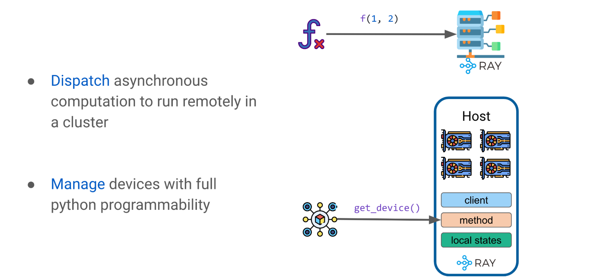 Figure 10: Ray patterns with Tasks and Actors
LinkAdvanced pattern: DeviceMesh
Earlier in the blog, we explained that in order to efficiently scale an LLM, we must partition model weights and computations on multiple GPU devices. Alpa utilizes Ray Actors to create more advanced device management abstractions such as a DeviceMesh: a two-dimensional mesh of GPU devices (see Figure 11).
A logical mesh can span multiple physical hosts, including all their GPU devices, with each mesh acquiring a slice of all GPUs on the same host. Multiple meshes can reside on the same host, and a mesh can even encompass an entire host. Ray Actors offer tremendous flexibility to manage GPU devices within a cluster.
For example, you can choose to have one actor per host, one per mesh, or even one per device depending on the level of orchestration control you require.
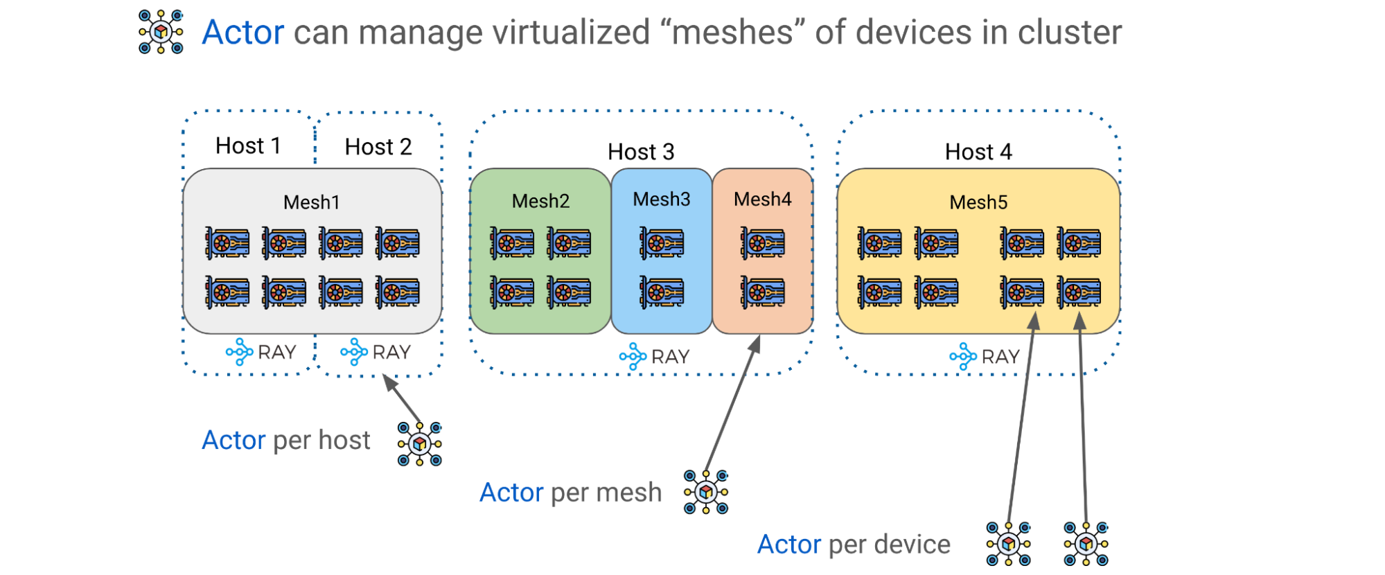 Figure 11: DeviceMesh for GPU cluster virtualization and management
LinkAdvanced pattern: GPU Buffers
The second advanced pattern in Alpa is GPU buffer management across DeviceMeshes. During GPU computations, we often end up with GPU tensors that represent tiles of a larger matrix. Alpa has an application-level GPU buffer management system that assigns a UUID for each GPU buffer and provides basic primitives, such as Send/Recv/Delete, to enable cross-mesh tensor movement and lifecycle management.
Using Ray Actors and DeviceMesh abstractions, buffers can be managed and transferred by invoking corresponding methods on the host to facilitate advanced model training paradigms.
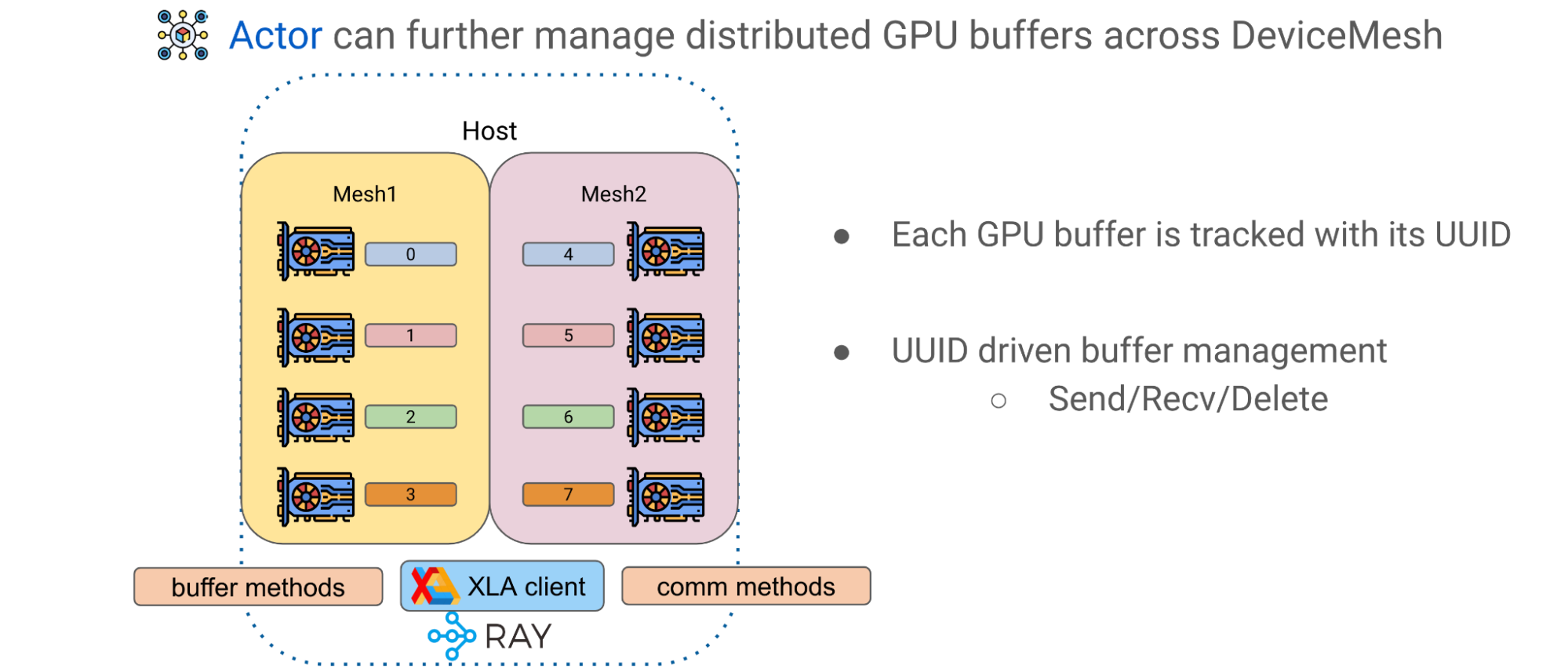 Figure 12: GPU buffer management with Ray Actor
LinkAdvanced pattern: Ray Collective
The third advanced pattern is Ray Collective, a collection of communication primitives that enables efficient and flexible tensor movement across different CPUs, GPUs and DeviceMesh(s). It is an essential communication layer for pipeline parallelism.
The simple intra-host case is depicted on the left side of figure 13 (Host 1), where GPU devices are interconnected with NVlink. The right side of figure 13 (Host 2 and 3) shows the multi-mesh, multi-host scenario, where communication occurs in a potentially more heterogeneous setup with a mix of intra-host NVLink and inter-host networking, such as InfiniBand, EFA, or Ethernet.
With Ray Collective, we can move and reshard tensors freely across DeviceMeshes via high-performance networking with NCCL, Nvidia’s Collective Communication Library for GPUs.
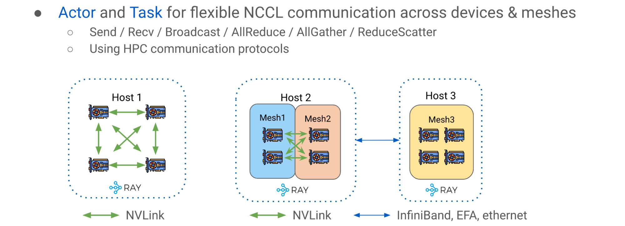 Figure 13: Ray Collective for cross mesh tensor movement via NCCL
LinkPipeline parallelism runtime orchestration
In JAX and Alpa, computations, communication, and instructions are often created to be static. The static artifact is an important property, because in JAX, a user program can be compiled to intermediate representations (IR) and then fed to XLA as a self-contained executable. Users can pass inputs into the executable and expect results as outputs, where all tensors are known in size and shape, just like a function for tensors.
The functional aspect of JAX and its lower level Intermediate Representation (IR) play nicely with Ray. If we revisit the Ray Task, where we decorate a function and let it execute in a cluster, the decorated function is the “executable.” In Ray, the executable is always produced by serializing the decorated Python function or class that wraps arbitrary code.
With JAX, however, the executable is a powerful unit of computation with clean mathematical properties. With good dispatching and orchestration of executables, we can represent complex and powerful neural networks, training paradigms such as transformers and pipeline parallelism, which is the essential technique imperative to scale LLM to GPU clusters.
Figure 14 is an end-to-end LLM pipeline parallelism example with Alpa on Ray. The end to end flow can be roughly divided into the following stages:
Inter-operator parallelism pass: Alpa optimally splits transformer blocks into separate pipeline stages and assigns them to respective DeviceMesh(es).
Intra-operator parallelism pass: Alpa partitions operator input and output matrices across GPU devices living on the same host along with GSPMD.
Generate static instructions for mesh workers: Compile a static executable for each DeviceMesh with respect to user configs such as pipeline schedule (1F1B, GPipe), micro batching, gradient accumulation, etc.
Each instruction can be {RUN, SEND, RECV, FREE} that handles running a self-contained JAX HLO/XLA program, allocate/transfer/free GPU buffer across DeviceMesh(es).
With static instructions, we greatly reduced scheduling frequency and overhead at Ray’s single controller level for better performance and scalability.
Put compiled executables into corresponding host Ray actors for later invocation.
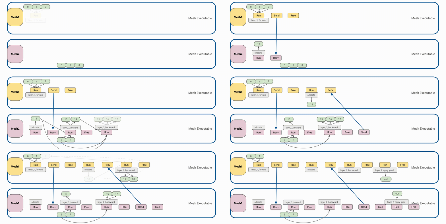 Figure 14: Example static instruction for two-layer pipeline parallelism
4. Driver calls and orchestrates compiled executables on each host worker to kick off end to end pipelined transformer training.
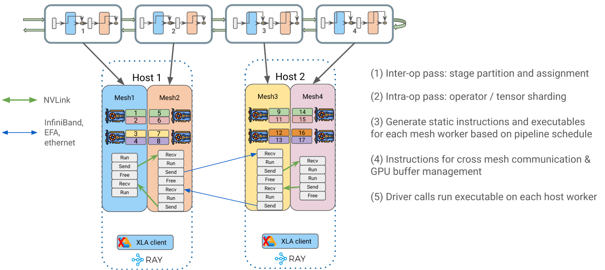 Figure 15: End to end pipeline parallelism runtime orchestration with Alpa on Ray
LinkRay on Alpa benchmark results
We closely collaborated with Nvidia to benchmark this effort for accurate performance results as well as scalability. For scalability and performance, the charts below, verified on an Nvidia’s Selene cluster, demonstrated total HW FLOPs throughput of OPT-175B with various GPU cluster sizes with peak HW FLOPs utilization of ~57.5% at ~179 TFLOPs/GPU. Model parallelization and partitioning are done automatically with a one-liner decorator.
Meta's original training of OPT-175B with PyTorch FSDP and manual Megatron-LM policy achieved ~147 TFLOPs/GPU in 2022. By contrast, Alpa on Ray achieved ~21.8% higher HW FLOPs without the requirement of implementing manual partitioning.
With respect to Benchmarks published by NVIDIA researchers on similar hardware, we achieved ~126 TFLOPs/GPU on NLG-530B in 2022, whereas Alpa on Ray achieved ~42% higher HW FLOPs.
Compared to Google’s internal PaLM-540B with Pathways, which achieved ~57.8% HW FLOPs utilization on TPUs in 2022, Alpa on Ray is very close to the efficiency of their internal implementation. However, we cannot make objective comparisons for benchmarks on different hardware – this is more of a reference.
These benchmark results strongly suggest that Alpa on Ray is one of the most performant and scalable frameworks for training LLM models in JAX, even at 175B scale. Furthermore, it’s capable of finding and executing optimal parallelization strategies automatically.
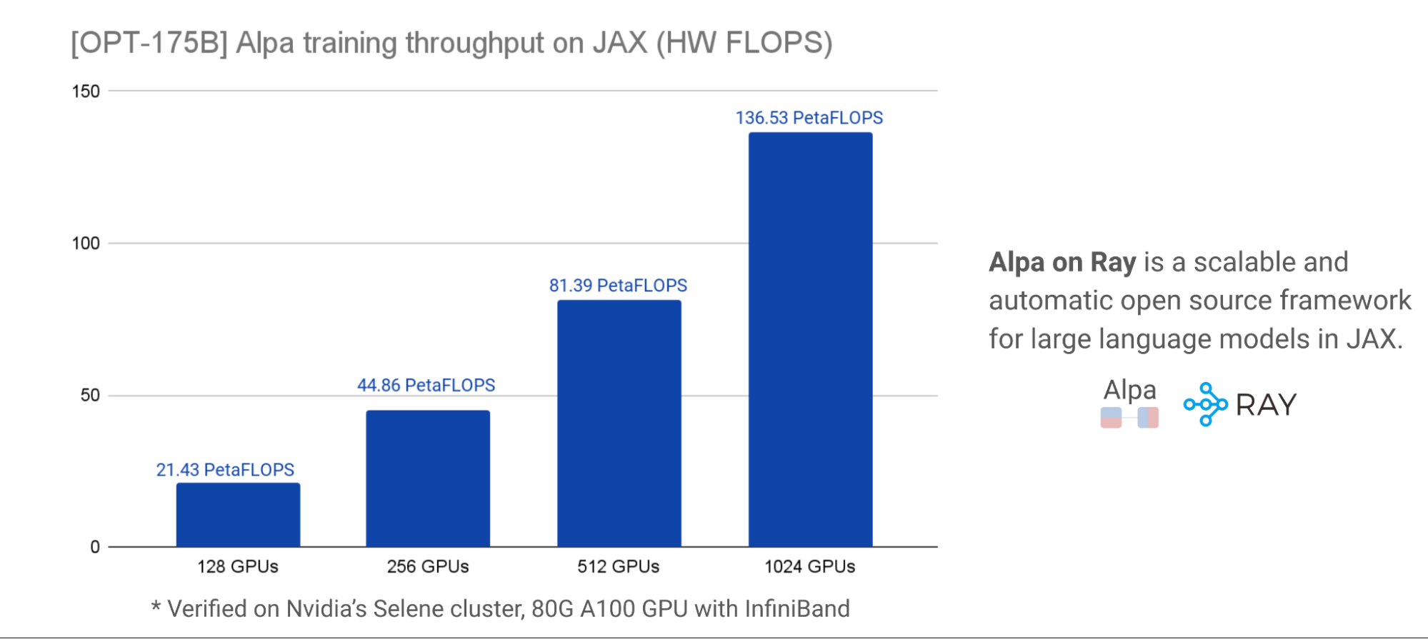 Figure 16: OPT-175B training throughput with Alpa on Ray, HW FLOPS
The above chart includes more details about the model definition and other configurations used to achieve the results. Refer to annotations at the bottom of figure for explanations.
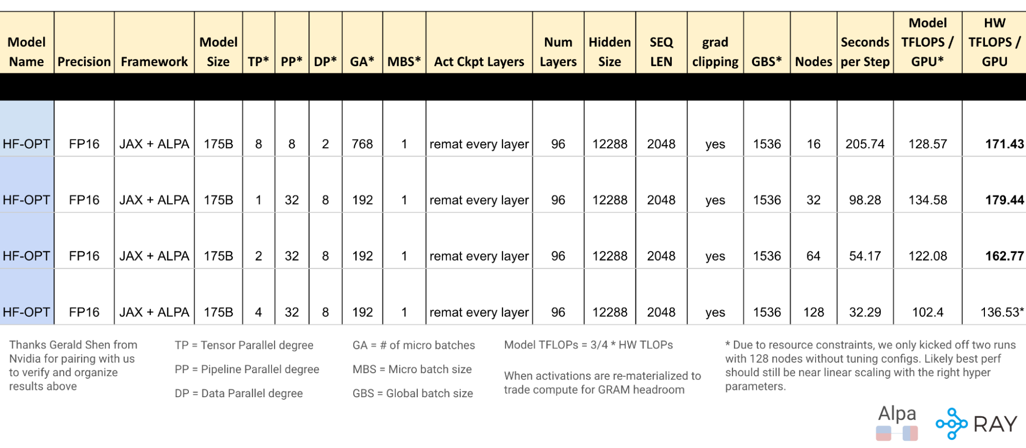 Figure 17: OPT-175B detailed config and metrics
LinkFuture improvements and considerations
A number of future improvements include:
Support for T5 with bf16 + pipeline parallelism at larger scale (We’ve enabled and benchmarked at 4 hosts scale within capacity constraint.)
Ease of use and production readiness improvements for the ML community
Further simplify LLM accessibility on commodity GPUs
LinkAcknowledgements
We (Alpa and Ray team) would like to thank AWS and CoreWeave for their generous support and sponsorship of working on A100 GPUs to facilitate our interactive development. Thank Nvidia for internal Selene cluster access for benchmarking at scale, as well as tremendous help for their partnership and support in this collaboration.
LinkNext Steps
For further exploration of Ray, Ray AIR*, and Ray on Alpa:
Read why we opine Ray as scalable compute is the right choice for LLM
Checkout the sources on GitHub
Checkout Ray documentation
Join our Ray monthly Ray Meetup, where we discuss all things Ray
Connect with the Ray community via forums: slack and discuss
Early-bird registration of Ray Summit 2023 is open. Grab your spot early
For further information of Alpa:
Checkout and star Alpa’s github for latest examples of LLM training and inference
Connect with the Alpa community via slack
We are sunsetting the "Ray AIR" concept and namespace starting with Ray 2.7. The changes follow the proposal outlined in this REP.


