We Pre-Trained Stable Diffusion Models on 2 billion Images and Didn't Break the Bank - Definitive Guides with Ray Series

This guide is the third in a series that will explore the challenges and solutions involved in training Stable Diffusion models at scale. Stable Diffusion models are a class of generative models that have shown promising results in generating high-quality images. However, training these models requires large amounts of data and computational resources, which can be challenging to manage. This guide will focus on the model training aspect of training Stable Diffusion models, particularly the challenges involved in running model training at scale.

In this guide, we will learn how to:

• 💻 Train a Stable Diffusion model using Ray Train + PyTorch Lightning

• 💡 Understand the strategies for optimizing the training process

• 🚀 Scale the training process to handle extensive datasets and computational demands

• 🔍 Identify common challenges faced during large-scale training and how to address them

LinkOverview

The code and algorithms behind Stable Diffusion are publicly available, allowing for model enhancement through training on high-quality datasets. Such training can improve image quality and address commercial use rights issues. However, training a diffusion model like Stable Diffusion from scratch requires a robust system for distributed computing. Without this, the training process could be lengthy and inefficient, leading to wasted time and resources.

Shown below is the end-to-end architecture diagram of the Stable diffusion model training. For reference, we already covered the Transformation and Encoding stages in the first guide, we aim to go over the training stage of the Stable Diffusion U-Net in this guide.

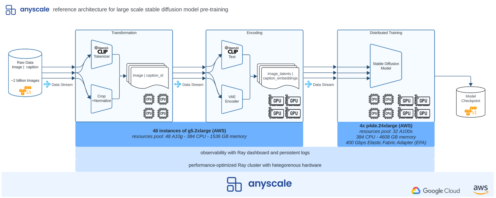Figure 1. End-to-end Stable Diffusion training architecture diagram.

Note that at any point in the above diagram we can choose to persist the data stream to storage and load it to complete the remainder stages. What we did in the first guide was to store the output of the “Encoding” stage to S3 so we have Stable Diffusion U-Net inputs ready. 

LinkGuide focus

Our approach is practical and code-oriented rather than deeply mathematical. We aim to equip you with the intuitive understanding necessary to adapt our code for your projects. The guide specifically focuses on implementing the model training stage for the v2-base model of Stable Diffusion.

LinkRequirements

You don't need access to a distributed computing cluster to follow and run the code in this guide, as the same code is compatible on both single machines and clusters, thanks to Ray’s versatility. If you are looking to scale your code, try the reference implementation on the Anyscale platform. What you will get is a VSCode remote session running within a minimally sized cluster.

LinkGuide progression

On a high level, the progression of this guide mimics the following steps needed to train a Stable Diffusion model, which we cover in much more detail later on:

1. Loading the preprocessed data: We start by loading the preprocessed data we prepared in our first guide.

2. Defining a Stable Diffusion model: Our Stable Diffusion model uses a network architecture called a U-Net. During training we start with preprocessed images (referred to as "image latents") and encoded text and iteratively add random noise to the image data ("noisy latents"). The U-Net will then learn to predict the noise we added. At inference time, we can then, for instance, start with a text description of an image we want to generate, and our Stable Diffusion model will invert the prior process (called a diffusion process), by iteratively subtracting noise from a completely random starting image, until the resulting image "looks like" text input we prompted the model with.

3. Defining a scalable training procedure: We scale the base model from the last step with Ray Train to enable running on a GPU compute cluster. We will go over how to set up and execute a Ray Train job, and how to integrate Ray Train with Ray Data to directly stream data onto the GPU training workers.

4. Running end-to-end training: Lastly, we show you how to carry out the training procedure itself on an Anyscale-managed Ray Cluster. We go over the specifics of the training process and discuss features like fault tolerance which Ray Train provides out of the box.

Let's start by loading the preprocessed data we prepared for training a Stable Diffusion model in the first guide.

LinkLoading precomputed image and text data from S3

We load our preprocessed dataset by implementing a simple load_precomputed_dataset function

1
2
3
4
5
6
7
8
9
10
11
12
13
14
15
16
17
18
19
def convert_precision_to_fp16(batch):
    for k, v in batch.items():
        batch[k] = v.astype(np.float16)
    return batch

def load_precomputed_dataset(
    data_uri: str, num_data_loading_workers: int, resolution: int = 256
) -> ray.data.Dataset:
    ds = ray.data.read_parquet(
        data_uri,
        columns=[f"image_latents_{resolution}", "caption_embeddings"],
        concurrency=num_data_loading_workers,
    )

    return ds.map_batches(
        convert_precision_to_fp16,
        batch_size=None,
        concurrency=num_data_loading_workers,
    )

load_precomputed_dataset will perform two steps:

1. Use ray.data.read_parquet to read the preprocessed image latents and caption embeddings 

   1. Ray Data adopts lazy execution and therefore this will simply return a Ray Dataset which represents our parquet dataset.

2. Apply convert_precision_to_fp16 to convert the data to a 16-bit floating point precision. 

   1. We chose to perform the precision halving on the data loading workers to reduce memory consumption on the training workers.

This is all we need to have our features ready for model training! As we will see later, Ray Train integrates seamlessly with Ray Data. Therefore no additional work is required in terms of constructing data loading functionality.

LinkDefining a Stable Diffusion model

Let's discuss the training process of a Stable Diffusion model in a bit more detail. Consider the following diagram as the basis for our discussion:

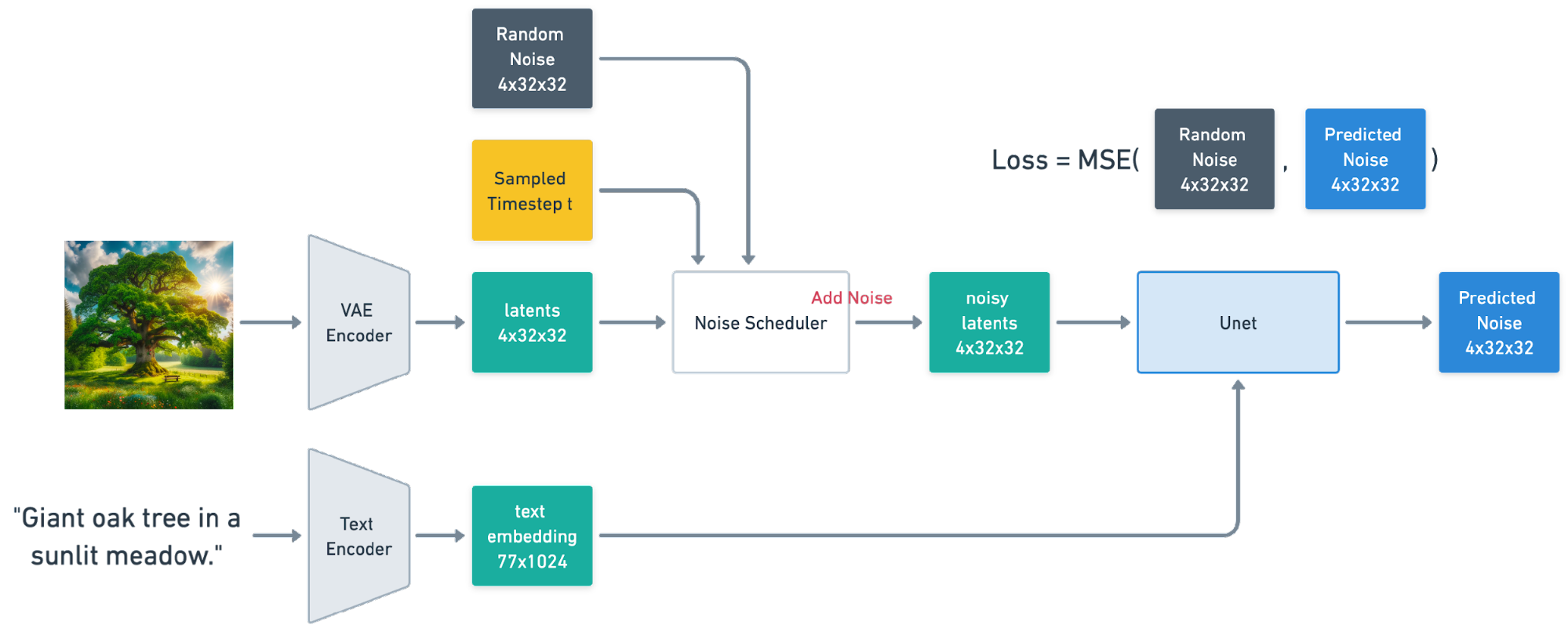Figure 2. Stable Diffusion model (U-Net) training.

The diagram contains a quick reminder of the preprocessing we applied: After cropping and normalizing images, we encoded them to a latent space using a VAE encoder. Tokenized text data is encoded with a CLIP model to generate text embeddings.

The core component of the training process is a U-Net, which we will define as a Pytorch Lighting module. The central idea of Stable Diffusion model training is to add random noise in image latent space at several timesteps t with a schedule, and apply it to get noisy latents. The purpose of U-Net is to learn to predict the noise. We compute the mean squared error (MSE) between the actual and the predicted noise as the loss function for training. Here's a visual representation of the full forward diffusion process as presented in the paper titled Denoising Diffusion Probabilistic Models.

Figure 3. Forward diffusion process. Picture taken from Denoising Diffusion Probabilistic Models.

As the U-Net gets better and better at predicting noise from noisy images, given an encoded text description, we can then use this to our advantage during inference. When provided with random noise and text input, we can instruct the U-Net to predict the noise, subtract it, and feed the result of it back into the U-Net, rinse and repeat. After a fixed number of steps we've removed "all the noise" and what's left is an image that fits the description. Here's a visual representation of the reverse diffusion process that leads to image generation:

Figure 4. Backward (reverse) diffusion process. Picture taken from Denoising Diffusion Probabilistic Models.

We're leaving out all mathematical details of this so-called diffusion process, but it is remarkable that learning to predictably destroy an image into pure noise means that you can predictably create art from pure noise, one iteration at a time. The idea of "just" chiseling away the random noise has a touch to it that is resembling the art of sculpting:

“The sculpture is already complete within the marble block, before I start my work. It is already there, I just have to chisel away the superfluous material.” Michelangelo

If you want to dive deep into the technical details of the diffusion process, we recommend you read the paper titled Denoising Diffusion Probabilistic Models.

LinkBuilding a LightningModule

Lets' define Stable Diffusion as a PyTorch Lightning module next. The definition itself is neither very difficult to understand, nor is it necessarily complex. But as the StableDiffusion class contains many methods, it ends up being a bit long. To prepare you for that, let's first inspect the interface to walk you through the process.

Overall, here is the interface of the StableDiffusion class:

1
2
3
4
5
6
7
8
9
10
11
12
13
14
15
16
17
18
class StableDiffusion(pl.LightningModule):
    def __init__(self, args):
        ...

    def on_fit_start(self):
        ...

    def forward(self, batch):
        ...

    def training_step(self, batch, batch_idx):
        ...

    def validation_step(self, batch, batch_idx):
        ...

    def configure_optimizers(self):
        ...

Let's break down the most important methods of StableDiffusion down, one by one.

Initialization:

We initialize a U-Net model and a noise scheduler in the __init__ method. A few things to note:

• The U-Net model config is fetched from the Hugginface Model Hub given a model name.

• The noise scheduler we chose to use is a Diffusion Denoising Probabilistic Model (DDPM) scheduler. 

  • The scheduler is responsible for sampling noise at different timesteps during training and we have loaded a pre-trained scheduler from the Huggingface Model Hub.

• The loss function is a simple mean square error loss function.

1
2
3
4
5
6
7
8
9
10
11
class StableDiffusion(pl.LightningModule):

    def __init__(self, model_name: str):
        model_config = PretrainedConfig.get_config_dict(model_name, subfolder="unet")
        self.unet = UNet2DConditionModel(**model_config[0])
        self.noise_scheduler = DDPMScheduler.from_pretrained(
            model_name, subfolder="scheduler"
        )
        self.loss_fn = F.mse_loss

    ...

Forward pass:

The forward pass of the model is defined in the forward method. Here, we perform the following:

1. Take the image latents and caption embeddings/latents as input

2. Sample noise at different timesteps

3. Add the noise to the image latents to get noisy latents

4. Pass the noisy latents through the U-Net model along with the encoded caption text to get the predicted noise

1
2
3
4
5
6
7
8
9
10
11
12
13
14
15
class StableDiffusion(pl.LightningModule):
    ...

    def forward(self, batch):
        image_latents = batch[f"image_latents_{self.resolution}"]
        caption_latents = batch["caption_embeddings"]

        timesteps = self._sample_timesteps(image_latents)
        noise = torch.randn_like(image_latents)
        noised_image_latents = self.noise_scheduler.add_noise(
            image_latents, noise, timesteps
        )

        outputs = self.unet(noised_image_latents, timesteps, caption_latents)["sample"]
        return outputs, noise

Training step:

The training_step method is where we compute the loss for the model. We calculate the mean squared error between the predicted noise and the actual noise. Pytorch Lightning will automatically perform the backward pass and the optimizer step with the returned loss.

1
2
3
4
5
6
7
class StableDiffusion(pl.LightningModule):
    ...

    def training_step(self, batch, batch_idx):
        outputs, targets = self.forward(batch)
        loss = self.loss_fn(outputs, targets)
        return loss

Configuring Optimizers

The configure_optimizers method is used to define the optimizer and learning rate scheduler for the model.

In this method, we define the optimizer and learning rate scheduler for the model. We use the get_linear_schedule_with_warmup function from the transformers library to create a linear learning rate scheduler with warmup. We also define the optimizer using the AdamW optimizer from the torch.optim module.

1
2
3
4
5
6
7
8
9
10
11
12
13
14
15
16
17
18
19
20
21
22
class StableDiffusion(pl.LightningModule):
    ...

    def configure_optimizers(self) -> OptimizerLRScheduler:
        optimizer = torch.optim.AdamW(
            self.trainer.model.parameters(),
            lr=self.lr,
            weight_decay=self.weight_decay,
        )
        scheduler = get_linear_schedule_with_warmup(
            optimizer,
            num_warmup_steps=self.num_warmup_steps,
            num_training_steps=self.num_training_steps,
        )
        return {
            "optimizer": optimizer,
            "lr_scheduler": {
                "scheduler": scheduler,
                "interval": "step",
                "frequency": 1,
            },
        }

get_linear_schedule_with_warmup creates a learning rate schedule with a warm up period during which it increases linearly from 0 to the initial lr set in the optimizer, and then decreases linearly from the initial lr set in the optimizer to 0 afterwards - see the figure below to visualize this.

Figure 5. Learning Rate Linear Schedule with Warm Up to lr=1.00, num_warmup_steps=100, num_training_steps=1000.

Note in our implementation, we increased num_training_steps to a very large number to maintain the initial_lr at an almost constant value after the warm up period. To view the full code implementing the StableDiffusion module, instantly provision a Ray cluster and start running your own download, check out the reference implementation on training Stable Diffusion on Anyscale.

LinkModel Training with PyTorch Lightning 

Now that we have defined the StableDiffusion model, we can define a PyTorch Lightning training script to train the model. A sample training code will look like the following:

1
2
3
4
5
6
7
8
9
10
11
12
13
14
15
16
17
18
19
20
21
22
23
24
25
26
27
def lightning_training_loop(
    init_from_pretrained: bool = False,
    model_name: str = "stabilityai/stable-diffusion-2-base",
    resolution: int = 256,
    lr: float = 1e-4,
    num_warmup_steps: int = 10_000,
    weight_decay: float = 1e-2,
    train_loader: DataLoader,
    val_loader: DataLoader,
) -> None:
    model = StableDiffusion(
        init_from_pretrained=init_from_pretrained,
        model_name=model_name,
        resolution=resolution,
        lr=lr,
        num_warmup_steps=num_warmup_steps,
        weight_decay=weight_decay,
    )

    trainer = pl.Trainer(
        accelerator="gpu",
        devices="auto",
        precision="bf16-mixed",
        strategy=FSDPStrategy(...),
        ...,
    )
    trainer.fit(model=model, train_dataloaders=train_loader, val_dataloaders=val_loader)

PyTorch Lightning provides a high-level interface for training PyTorch models. The Trainer class is used to configure and run the training loop. The fit method is used to train the model on the training data and validate it on the validation data. The training loop above requires data loaders to be prepared which we will not go into detail here as we will focus on producing data loaders from Ray Data when we scale the training process.

LinkDefining a scalable training procedure

LinkOverview of Ray Train

To scale our training with Ray Train, our resulting code will look like something like this:

1
2
3
4
5
6
7
8
9
10
11
12
13
14
15
16
from ray.train import TorchTrainer

def train_func(config):
    ...

trainer = TorchTrainer(
    train_func,
    scaling_config=ScalingConfig(num_workers=num_workers, use_gpu=True),
    run_config=RunConfig(
        name=experiment_name,
        storage_path=storage_path,
        failure_config=FailureConfig(max_failures=max_failures),
    ),
    datasets=ray_datasets,
)
trainer.fit()

We perform two main steps in the code above:

1. Instantiate a trainer by using the  ray.train.TorchTrainer class which ties together the following components:

   • train_func: A Python function that contains our model training logic. train_func will be a slightly modified version of the lightning_training_loop we defined earlier as we will see below.

   • scaling_config: An object specifying the number of workers and whether to use GPUs. For more complex resource configurations, see the docs page here

   • run_config: A configuration of the experiment, storage settings, and the maximum number of failures allowed.

   • datasets: A Python dictionary of training and validation Ray Dataset objects that will be used for training the model.

2. Call trainer.fit to launch workers on the Ray cluster, distribute the training function to the workers, and launch a process to manage the training job. Here's a high-level overview of the process:

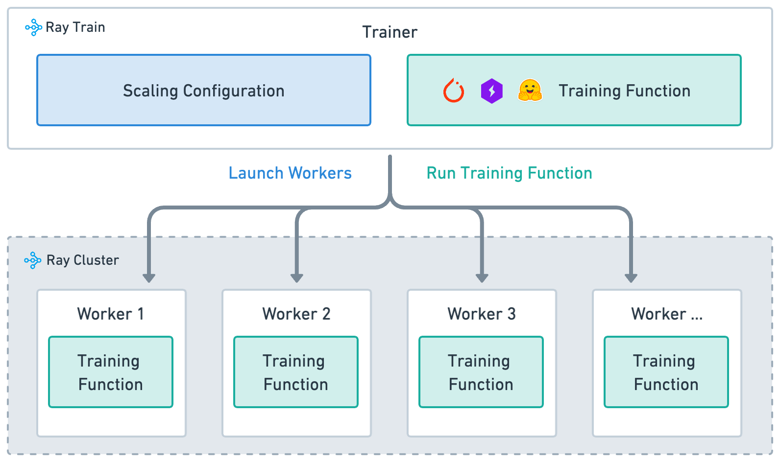Figure 6. Overview of distributed training with Ray Train.

LinkData Loading and Preprocessing

Ray Train integrates with Ray Data to offer a performant and scalable streaming solution for loading and preprocessing large datasets. By default, Ray Data shards all datasets across workers as shown in the diagram below:

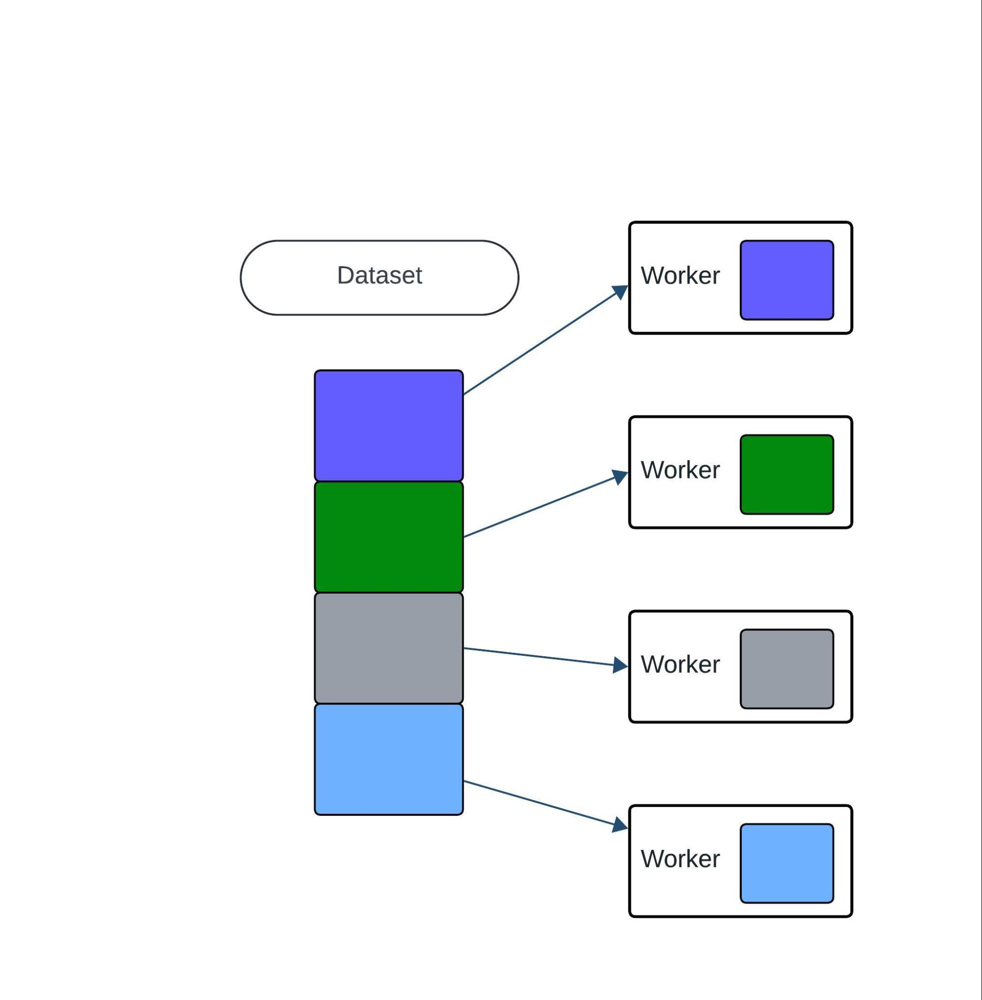Figure 7. A Ray Data Dataset is split equally across the training workers by default.

To access the ray_datasets we passed to our TorchTrainer  from within a worker's training function, we make use of the method get_dataset_shard from Ray Train. To generate data loaders from the Ray datasets, we use the iter_torch_batches method. Here's how we our train_func will handle data loading and preprocessing:

1
2
3
4
5
6
7
8
9
10
11
12
13
14
15
16
17
18
19
20
21
22
def train_func(config):
    train_ds = train.get_dataset_shard("train")
    val_ds = train.get_dataset_shard("validation")

    train_dataloader = train_ds.iter_torch_batches(
        batch_size=config["batch_size"]
    )
    val_dataloader = val_ds.iter_torch_batches(
        batch_size=config["batch_size"]
    )

    ...

    trainer = pl.Trainer(
        ...
    )

    trainer.fit(
        model,
        train_dataloaders=train_dataloader,
        val_dataloaders=val_dataloader
    )

LinkLast mile preprocessing on the training worker

In case you need to perform some last-mile preprocessing on the training worker, you can use the collate_fn argument in iter_torch_batches. This function will be called on each worker to preprocess the data before it is fed into the model. Here's how we will use the collate_fn argument to move the data to the GPU:

1
2
3
4
5
6
7
8
9
10
11
12
13
14
15
16
17
18
19
20
21
22
23
24
def move_to_device_collate_fn(batch, device):
    for k, v in batch.items():
        batch[k] = torch.tensor(v).to(device)
    return batch

def train_func(config):
    ...

    collate_fn = partial(
        move_to_device_collate_fn,
        device=ray.train.torch.get_device()
    )
    train_dataloader = train_ds.iter_torch_batches(
        batch_size=config["batch_size"],
        collate_fn=move_to_device_collate_fn,
        prefetch_batches=config["num_batches_to_prefetch"],
        ...
    )
    val_dataloader = val_ds.iter_torch_batches(
        batch_size=config["batch_size"],
        collate_fn=move_to_device_collate_fn,
        prefetch_batches=config["num_batches_to_prefetch"],
        ...
    )

Note given the collate_fn operation happens locally in the training workers we avoid adding any heavy transformation in this function as it may become the bottleneck. Additionally, we can further reduce bottlenecks by passing iter_torch_batches a prefetch_batches argument. If prefetch_batches is set to N, Ray Train will launch background threads to fetch and process the next N batches.

LinkDefining the training function

Having shown how to load the data within a training function, let's now define the main training function that we will use to train the Stable Diffusion model using Ray Train. The training function will perform the following steps:

1. Initialize random seeds for reproducibility

2. Load the training and validation datasets

3. Initialize the Stable Diffusion model

4. Initialize the PyTorch Lightning Trainer

5. Train the model

1
2
3
4
5
6
7
8
9
10
11
12
13
14
15
16
17
18
19
20
21
22
23
24
25
26
27
28
29
30
31
32
33
34
35
def train_func(config: dict):
    pl.seed_everything(config["seed"])
    ...
    train_dataloader = train_ds.iter_torch_batches(
        batch_size=config["batch_size_per_worker"],
        collate_fn=collate_fn,
        ...
    )
    validation_dataloader = validation_ds.iter_torch_batches(
        batch_size=config["batch_size_per_worker"],
        collate_fn=collate_fn,
        ...
    )
    model = StableDiffusion(
        init_from_pretrained=config["init_from_pretrained"],
        model_name=config["model_name"],
        resolution=config["resolution"],
        lr=config["lr"],
	 ...
    )
    ...
    trainer = pl.Trainer(
        accelerator="gpu",
        precision="bf16-mixed",
        strategy=RayFSDPStrategy() if config["fsdp"] else RayDDPStrategy(),
        plugins=[RayLightningEnvironment()],
        callbacks=callbacks,
        ...
    )

    trainer.fit(
        model,
        train_dataloaders=train_dataloader,
        val_dataloaders=validation_dataloader,
    )

LinkDistributed training strategies: evaluating DDP vs FSDP 

You might have noticed that we specified a distribution strategy in our above training function as either RayFSDPStrategy or RayDDPStrategy. Fully Sharded Data Parallelism (FSDP) and Distributed Data Parallelism (DDP) are two strategies used in distributed machine learning training to handle large models and datasets by distributing the workload across multiple machines. While both aim to improve training efficiency and scalability, they employ different approaches to achieve these goals.

In general, the choice between Distributed Data Parallelism (DDP) and Fully Sharded Data Parallelism (FSDP) in distributed training typically depends on the specific requirements of your training job, such as model size, resource constraints, and scalability needs. Both methods have their advantages and scenarios where they perform best. Here’s a breakdown to help you choose the right strategy:

LinkDistributed Data Parallelism (DDP)

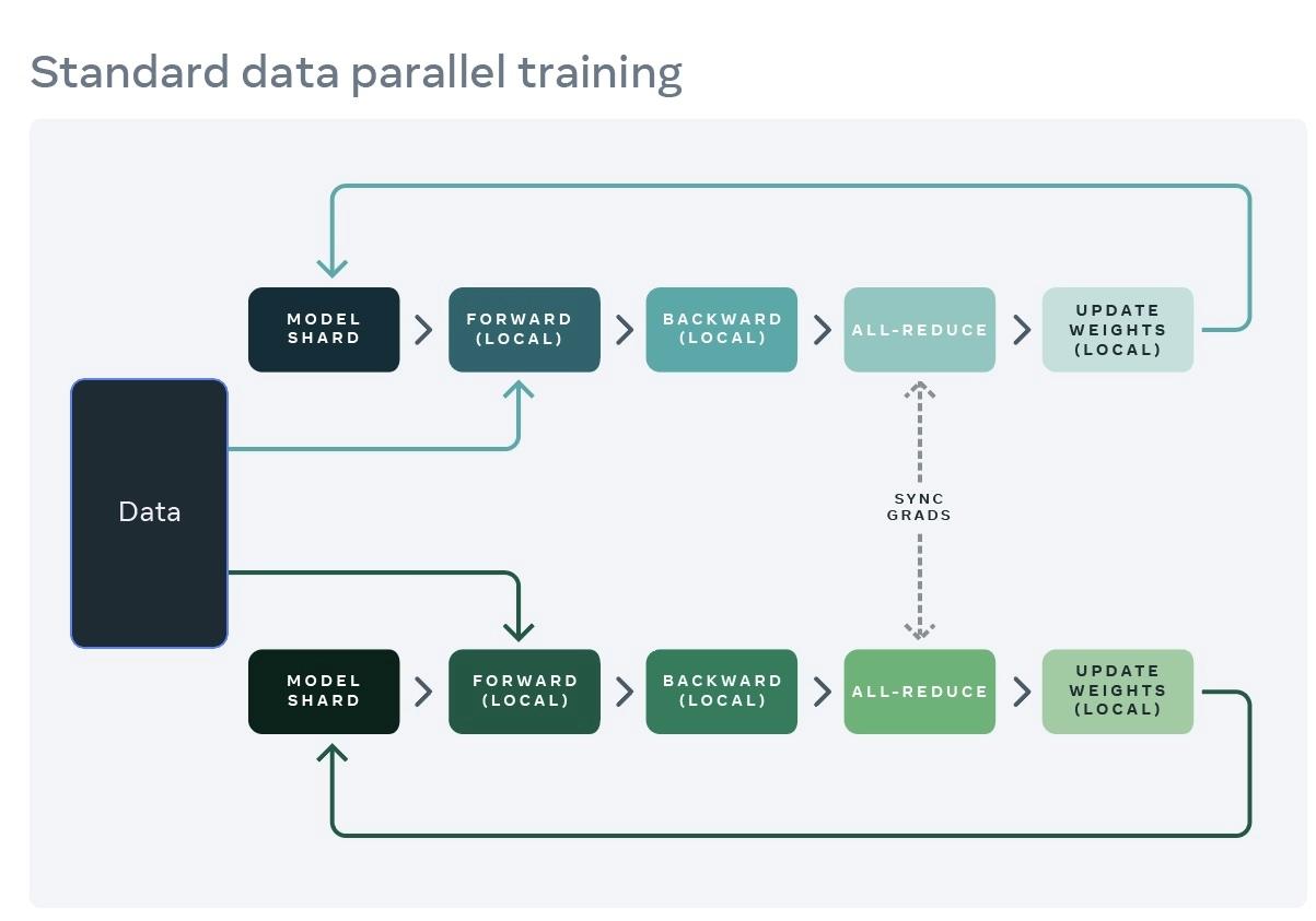
Figure 8: Distributed Data Parallelism (DDP) in distributed training. Picture taken from the facebook engineering blog post on FSDP

How it Works:

DDP is one of the most straightforward and commonly used strategies for distributed training. It replicates the entire model on each GPU or node in the cluster, with each replica working on a different subset of the data. 

The core idea is to parallelize the training by distributing data batches across different nodes, where each node computes gradients independently. After each backward pass, DDP synchronizes gradients across all nodes to update the model weights consistently. This approach is relatively simple to implement and can significantly speed up training for large datasets.

Advantages:

• Simplicity: It is easier to implement and integrate with existing models because each process handles a complete copy of the model.

• Performance: Typically, DDP offers good speedup and performance, especially when the communication overhead is managed (e.g., with efficient collective communication primitives).

Disadvantages:

• Memory Utilization: Each GPU needs memory for a full model copy, which can be inefficient for very large models.

• Scaling Limit: As model sizes grow, the memory requirement can become a bottleneck.

LinkFully Sharded Data Parallelism (FSDP)

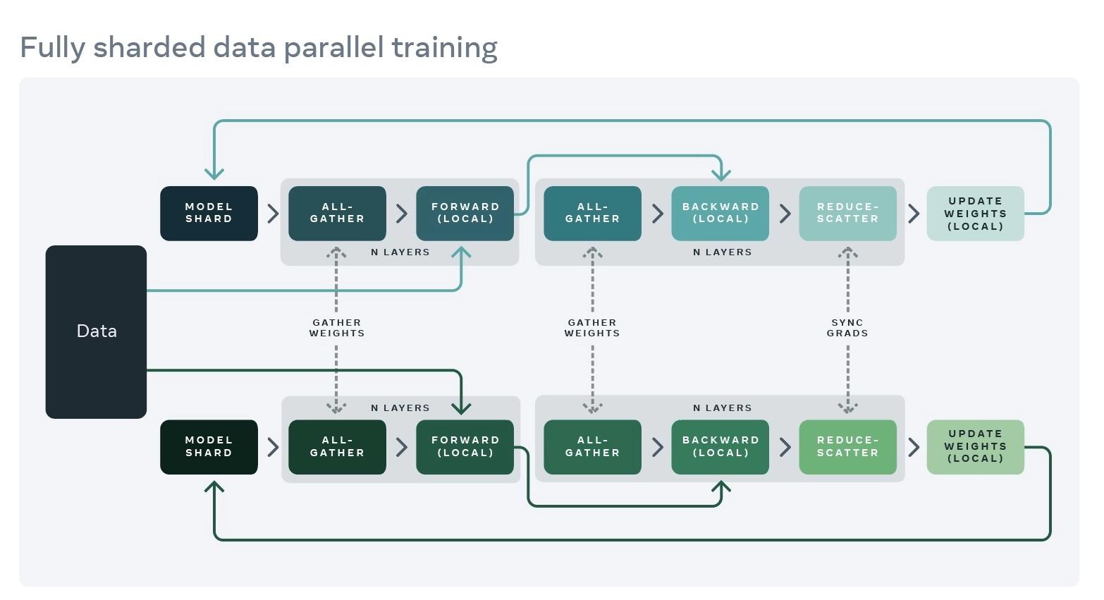
Figure 9: Fully Sharded Data Parallelism (FSDP) in distributed training in FULL_SHARD mode. Picture taken from the facebook engineering blog post on FSDP

How it Works: FSDP takes a different approach to distributed training by sharding (splitting) both the data and any of the following across all available GPUs:

• Optimizer states

• Gradients 

• Model parameters

The extent of “model-based sharding” is configurable in lightning. The available sharding configurations include:

• FULL_SHARD: Shards model parameters, gradients, and optimizer states (default).

• SHARD_GRAD_OP: Shards gradients and optimizer states only. Model parameters get replicated.

• NO_SHARD: No sharding (similar to regular DDP).

• HYBRID_SHARD: Shards model parameters, gradients, and optimizer states within a single machine, but replicates across machines.

Advantages:

• Memory Efficiency: Greatly reduces the memory footprint on each GPU for large models, which allows training much larger models or increasing the batch size.

Disadvantages:

• Development Complexity: More complex to configure and debug, especially when using other optimizations together with it.

LinkChoosing Between DDP and FSDP

• Model Size: If your model fits comfortably in the memory of a single GPU, DDP is typically sufficient and easier to manage. For very large models that exceed GPU memory limits, FSDP is likely necessary.

• Resource Availability: If you have access to a large number of GPUs and need to optimize memory usage, FSDP can be more advantageous.

• Development Complexity: DDP is simpler to configure and debug. If your team is smaller or less experienced with distributed systems, starting with DDP might be preferable.

• Training Time and Efficiency: Consider the training time and scalability needs. FSDP can sometimes be slower per iteration but allows for training larger models or using larger batch sizes, which can be a critical factor.

In summary, no one strategy is always clearly better than the other. The choice largely depends on the specific constraints and requirements of your training workload. In many practical scenarios, teams might start with DDP due to its simplicity and lower barrier to entry, and move to FSDP as model sizes and scaling needs grow.

In our specific case, we found that FSDP in SHARD_GRAD_OP mode was the best choice for training Stable Diffusion models striking a balance between a more efficient use of GPU memory and increased communication overhead, see our blog post for more details.

LinkBuilding a training script

Finally, we can define the train script as follows:

1
2
3
4
5
6
7
8
9
10
11
12
13
14
15
16
17
18
19
20
21
22
23
24
25
26
27
28
29
30
31
32
33
34
35
36
37
38
39
40
41
42
43
44
45
46
47
48
49
50
51
52
53
54
55
56
57
58
59
60
61
...

@app.command
def train(
    storage_path: str,
    train_data_uri: str,
    validation_data_uri: str,
    experiment_name: str = "exp-base",
    model_name: str = "stabilityai/stable-diffusion-2-base",
    init_from_pretrained: bool = False,
    resolution: int = 256,
    lr: float = 1e-4,
    weight_decay: float = 1e-2,
    max_steps: int = -1,
    num_warmup_steps: int = 10000,
    batch_size_per_worker: int = 32,
    num_data_loading_workers: int = 16,
    num_training_workers: int = 16,
    seed: int = 420,
    max_failures: float = 0,
):

    ray_datasets = {
        "train": load_precomputed_dataset(
            data_uri=train_data_uri,
            resolution=resolution,
            num_data_loading_workers=num_data_loading_workers,
        ), 
        "validation": load_precomputed_dataset(
            data_uri=validation_data_uri,
            resolution=resolution,
            num_data_loading_workers=num_data_loading_workers,
        )
    }

    trainer = TorchTrainer(
        train_func,
        train_loop_config={
            "model_name": model_name,
            "resolution": resolution,
            "lr": lr,
            "weight_decay": weight_decay,
            "init_from_pretrained": init_from_pretrained,
            "seed": seed,
            "batch_size_per_worker": batch_size_per_worker,
            "max_steps": max_steps,
            "num_warmup_steps": num_warmup_steps,
            "project_name": experiment_name,
        },
        scaling_config=ScalingConfig(
            num_workers=num_training_workers, use_gpu=True
        ),
        run_config=RunConfig(
            name=experiment_name,
            storage_path=storage_path,
            failure_config=FailureConfig(max_failures=max_failures),
        ),
        datasets=ray_datasets,
    )

    trainer.fit()

The train script is a command-line interface that allows you to run the training process on a Ray cluster. The script takes in various arguments such as the storage path, training and validation data URIs, experiment name, model name, and other hyperparameters. The script then uses the TorchTrainer class to combine all the components we discussed earlier and calls trainer.fit to run the training process on a Ray cluster.

To view the full code implementing the train script, instantly provision a Ray cluster and start running your own download, check out the reference implementation on training stable diffusion on Anyscale.

LinkA note on fault tolerant training

Here's an illustration of how experiment restoration works in Ray Train:

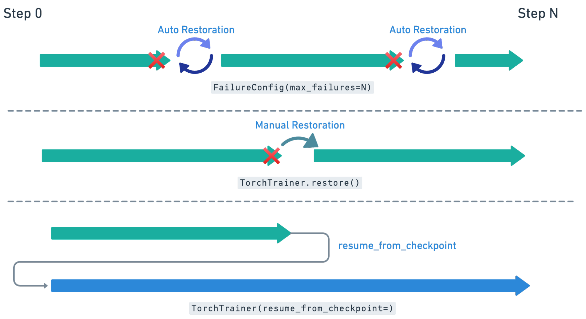
Ray Train has built-in fault tolerance to recover from worker failures (i.e. RayActorErrors). When a failure is detected, the workers will be shut down and new workers will be added in. The training function will be restarted, but progress from the previous execution can be resumed through checkpointing. 

In order to retain progress when recovery, the training function must implement logic for both saving and loading checkpoints. Each instance of recovery from a worker failure is considered a retry. The number of retries is configurable through the max_failures attribute of the FailureConfig argument set in the RunConfig passed to the Trainer.

Here is how we would update out train_func to save and recover from a checkpoint

1
2
3
4
5
6
7
8
9
10
11
12
13
14
15
16
def train_func():
# Recover from checkpoint
	if ray.train.get_checkpoint():
		...	

	for i in range(num_epochs):
		...
	# Save a checkpoint
	ray.train.report(metrics, checkpoint)

trainer = TorchTrainer(
	...
	failure_config=FailureConfig(
		max_failures=-1
)
)

To manually restore a training job, you can use the restore method of the Trainer class. This method will restore the training job from the last checkpoint and continue training from that point.

LinkOffline vs. Online preprocessing

So far our implementation can be summarized with the following diagram:

We performed the preprocessing and stored the dataset on S3. That means to use this processed data for Stable Diffusion training, we then have to pick it up again and feed it into the Unet-model that's central to all Stable Diffusion models. This approach is also known as “Offline preprocessing”.

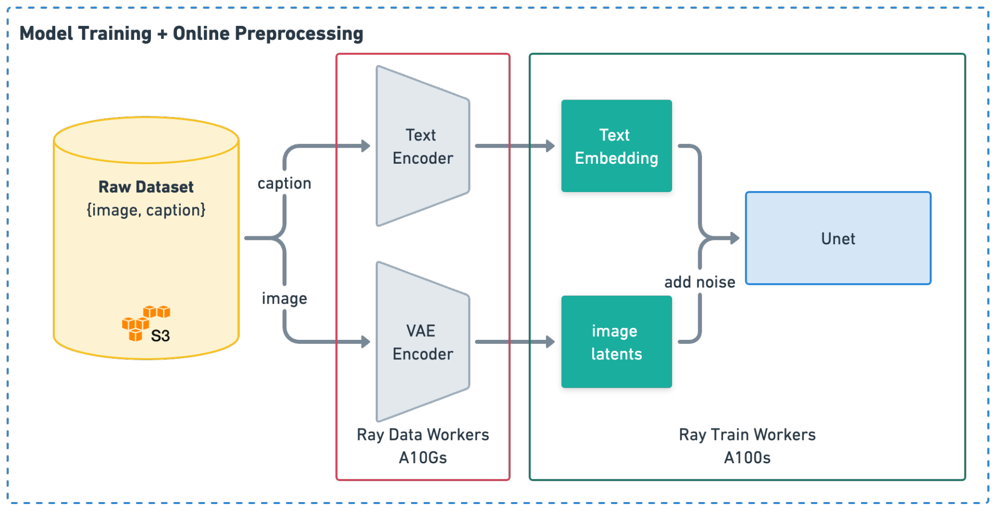
The alternative to this approach is to preprocess the raw LAION data online - i.e. "on the fly" before feeding it into an Stable Diffusion model for training. This way, we can "merge" preprocessing and training into a single end-to-end pipeline in a Ray cluster. Schematically, online preprocessing looks like this:

LinkConsiderations for Offline Preprocessing

You might want to perform offline preprocessing for these reasons:

• Cost Efficiency: Preprocessing data in advance allows for reuse in multiple training runs, reducing the need for repeated pre-processing and potentially lowering overall costs.

  • Note: This assumes preprocessing is deterministic, which may not apply if you want to perform transformations like random image cropping in your custom training of Stable Diffusion.

• Simplified Optimization: Enables full focus on enhancing the training process itself, such as maximizing GPU utilization, without the overhead of coupling to pre-processing.

Challenges include higher storage costs due to the need to save processed data, and less flexibility since adjustments require rerunning the entire preprocessing.

LinkConsiderations for Online Preprocessing

Consider online preprocessing for:

• Ideal for Dynamic Preprocessing: A natural choice when dynamic, on-the-fly adjustments to preprocessing steps are necessary.

• Immediate Training Start: Training can begin as soon as raw data is available, eliminating preprocessing wait times.

However, this method may increase the complexity of managing resources and can lead to higher operational costs if data needs frequent reprocessing for each training session.

Read our blog post to better quantify the above trade-offs between offline and online preprocessing and choose the right approach for your use case.

LinkImplementing Online preprocessing

If we want to implement online preprocessing, the change is simple enough with Ray Data. Instead of making use of the load_precomputed_dataset to fetch our training and validation data. We will make use of the get_laion_streaming_dataset method that we implemented in our first guide to which implemented the core logic for preprocessing.

Therefore here is what will change in our train script:

1
2
3
4
5
6
7
8
9
10
11
12
13
14
15
16
17
18
19
20
21
22
23
24
25
26
27
28
29
30
31
32
33
34
35
36
37
38
39
40
41
42
43
...

@app.command
def train(
    storage_path: str,
    online_preprocessing: bool,
    processed_train_data_uri: str | None,
    processed_validation_data_uri: str | None,
    resolution: int = 256,
    batch_size_per_worker: int = 32,
    num_enconders: int = 16,
    num_data_loading_workers: int = 16,
    ...
):
    if online_preprocessing:
        ray_datasets = {
            "train": get_laion_streaming_dataset(
                input_uri=raw_train_data_uri,
                batch_size=batch_size_per_worker,
                resolution=resolution,
                num_encoders=num_enconders,
            ),
            "validation": get_laion_streaming_dataset(
                input_uri=raw_validation_data_uri,
                batch_size=batch_size_per_worker,
                resolution=resolution,
                num_encoders=num_enconders,
            ),
        }
    else:
        ray_datasets = {
            "train": load_precomputed_dataset(
                data_uri=processed_train_data_uri,
                resolution=resolution,
                num_data_loading_workers=num_data_loading_workers,
            ),
            "validation": load_precomputed_dataset(
                data_uri=pocessed_validation_data_uri,
                resolution=resolution,
                num_data_loading_workers=num_data_loading_workers,
            ),
        }
    ...

LinkKey Takeaways

In this guide, we learned the following:

• How to train a Stable Diffusion model using Ray Train + PyTorch Lightning

• How to assess online vs. offline preprocessing and integrate Ray Data for our training pipeline

• How to scale the training process to handle extensive datasets and computational demands

LinkFuture work

In future guides, we aim to show the implementation in Ray for training more recent versions of Stable Diffusion models such as Stable Diffusion V3 which entail even more challenging resource data processing requirements.

LinkConclusion

Training Stable Diffusion models at scale can be a challenging task due to the large amounts of data and computational resources required. Ray Train provides a powerful framework for distributed training that can help you efficiently train Stable Diffusion models on large datasets. By following the steps outlined in this guide, you can train Stable Diffusion models at scale and take advantage of the benefits of distributed training.

To view the full code implementing the end-to-end training process, instantly provision a Ray cluster and start running your own download, check out the reference implementation on training stable diffusion on Anyscale.