Processing 2 Billion Images for Stable Diffusion Model Training - Definitive Guides with Ray Series

This guide is the second in a series that will explore the challenges and solutions involved in training Stable Diffusion models at scale. Stable Diffusion models are a class of generative models that have shown promising results in generating high-quality images. However, training these models requires large amounts of data and computational resources, which can be challenging to manage. This guide will focus on the data processing aspect of training Stable Diffusion models, particularly the challenges involved in preparing training data at scale.

In this guide, we will learn how to:

• 💻 Develop an end-to-end data processing pipeline for Stable Diffusion model training.

• 🚀 Build scalable data pipelines that you can apply to handle petabyte-scale datasets.

• 💡 Familiarize yourself with Ray, an open-source tool for scalable computing.

• 🔍 Dive deep into optimizing Ray Data for loading and processing large datasets efficiently.

LinkOverview

Diffusion models like Stable Diffusion, Sora, and DALL-E excel in generating detailed, high-quality creative outputs. Notably, Stable Diffusion is open-source and crafts images from text descriptions, making it a pivotal tool in AI-driven art and design.

Prompt: "Sunrise over a Scottish landscape". Figure 1: Example text-to-image output of a Stable Diffusion model.

Stable Diffusion's openly available code and algorithms encourage enhancements through training on high-quality datasets. Such training can improve image quality and address commercial usage rights. Yet, building a diffusion model from scratch demands significant computing resources, potentially leading to lengthy and inefficient training periods without robust distributed computing systems.

LinkGuide focus

Our approach is practical and code-oriented rather than deeply mathematical. We aim to equip you with the intuitive understanding necessary to adapt our code for your projects. The guide specifically focuses on preparing data for the v2-base model of Stable Diffusion.

LinkRequirements

You don't need access to a distributed computing cluster to follow and run the code in this guide, as the same code is compatible on both single machines and clusters, thanks to Ray’s versatility. If you are looking to scale your code, try the reference implementation on the Anyscale platform. What you will get is a VSCode remote session running within a minimally sized cluster.

LinkGuide progression

On a high level, the progression of this guide mimics the following steps needed to prepare training data for a Stable Diffusion model, which we cover in much more detail later on:

1. Download the right dataset: There are various interesting subsets of the so-called LAION dataset that is commonly used in Stable Diffusion training. The data consists of a collection of images and their text descriptions.

2. Transform the data: Both the images and the text from the LAION data need to be processed for the Stable Diffusion training procedure. The first step is to crop and clean the images from the raw dataset and tokenize the text.

3. Encode the data: Then both images and text need to be suitably encoded. We send the images through the encoding step of a variational autoencoder and the tokenized text through the encoding step of a Contrastive Language-Image Pretraining (CLIP) model.

Let's download some data next to get started!

LinkDownloading LAION datasets

The Large-scale Artificial Intelligence Open Network (LAION) non-profit organization publishes models and datasets under a public license. LAION is particularly known for having provided the data underlying practically most Stable Diffusion models (see the v2-base model card for more details). The community sometimes colloquially refers to "the LAION dataset", but there are really a lot of datasets available.

For this guide, we are primarily interested in the LAION Aesthetic dataset, which is a subset of the larger LAION 5B dataset selected for aesthetic images. It consists of image and text pairs. Here are a couple of examples:

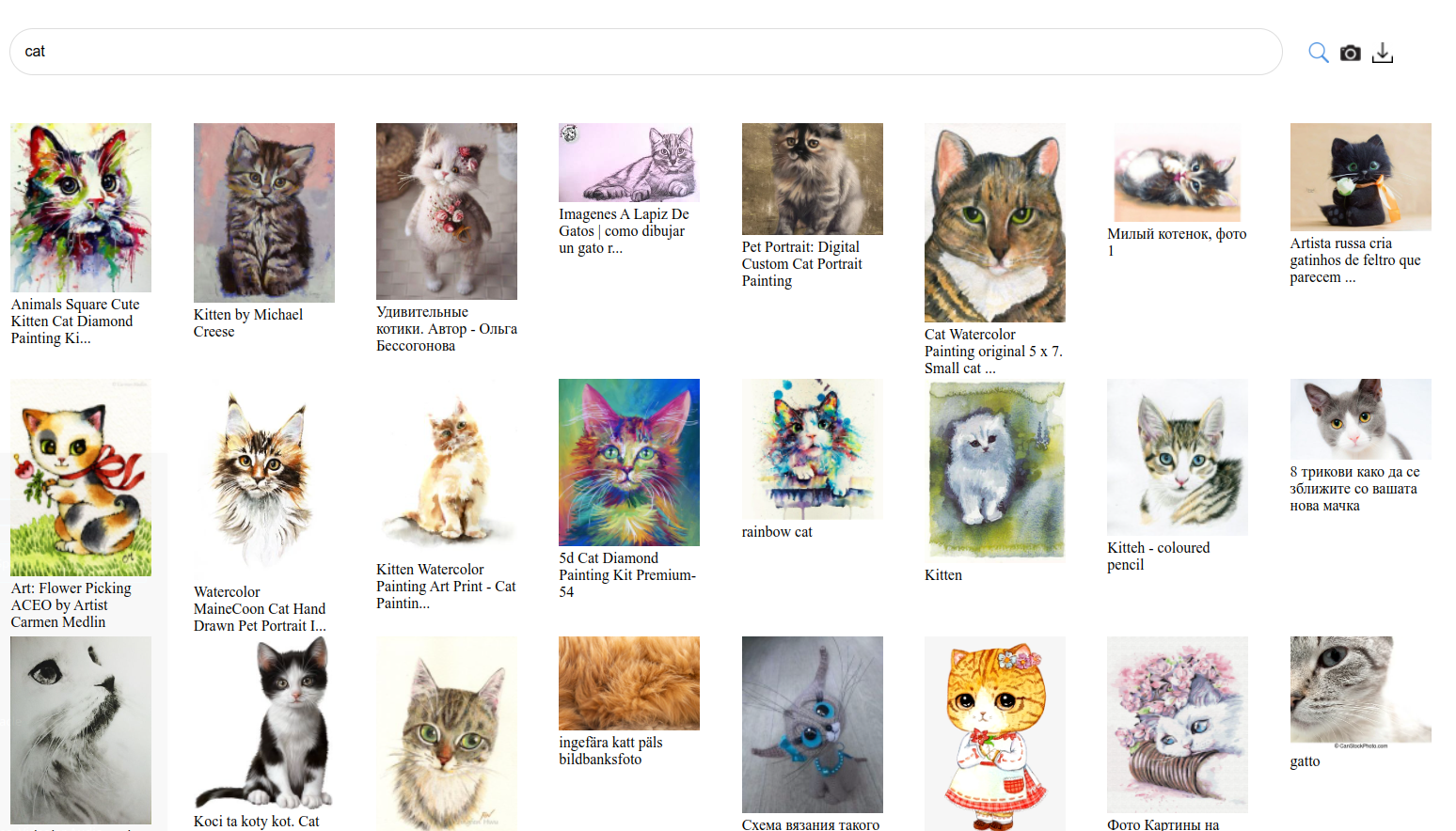
Figure 2: Cat images in the LAION Aesthetic dataset - picture taken from the LAION-datasets github repo.

NOTE: Access to LAION datasets on HuggingFace has recently been disabled. This is due to an ongoing safety review of LAION 5B. If you would like to skip the download logic, you can move directly to the section titled "Processing Image and Text Data”. However, we recommend that you still go through the download code to get a better understanding of how to do so efficiently. In any case, we'll help you circumvent this temporary issue by providing S3 buckets for raw and processed data, so that you can run all other code in a frictionless manner. 

LinkDownloading the dataset with Ray Data

There are community-contributed command line tools like img2dataset that can help you download LAION data, too. In fact, it's the tool recommended by the LAION team on GitHub. However, img2dataset can only save files to a local machine. To store files on a remote storage like AWS S3, you will need to run a sync operation. 

Ray Data provides an efficient way to distribute download workloads across a Ray cluster. It can directly stream data to S3 without going through an intermediary file system; all operations are performed in the memory of the nodes within the cluster.

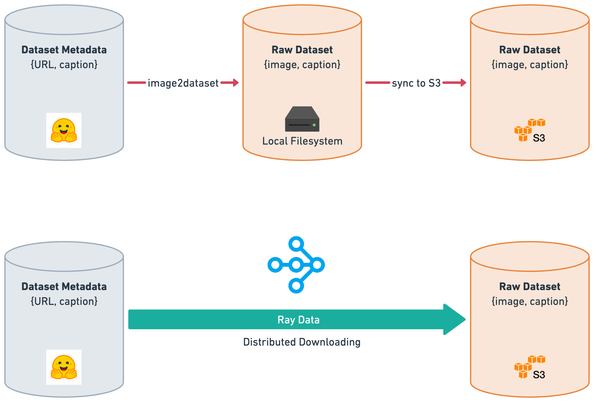Figure 3: Distributed downloading with img2dataset (shown as image2dataset) vs Ray Data.

LinkArchitecture Overview

Here's a high-level overview of the download process that we would like to implement:

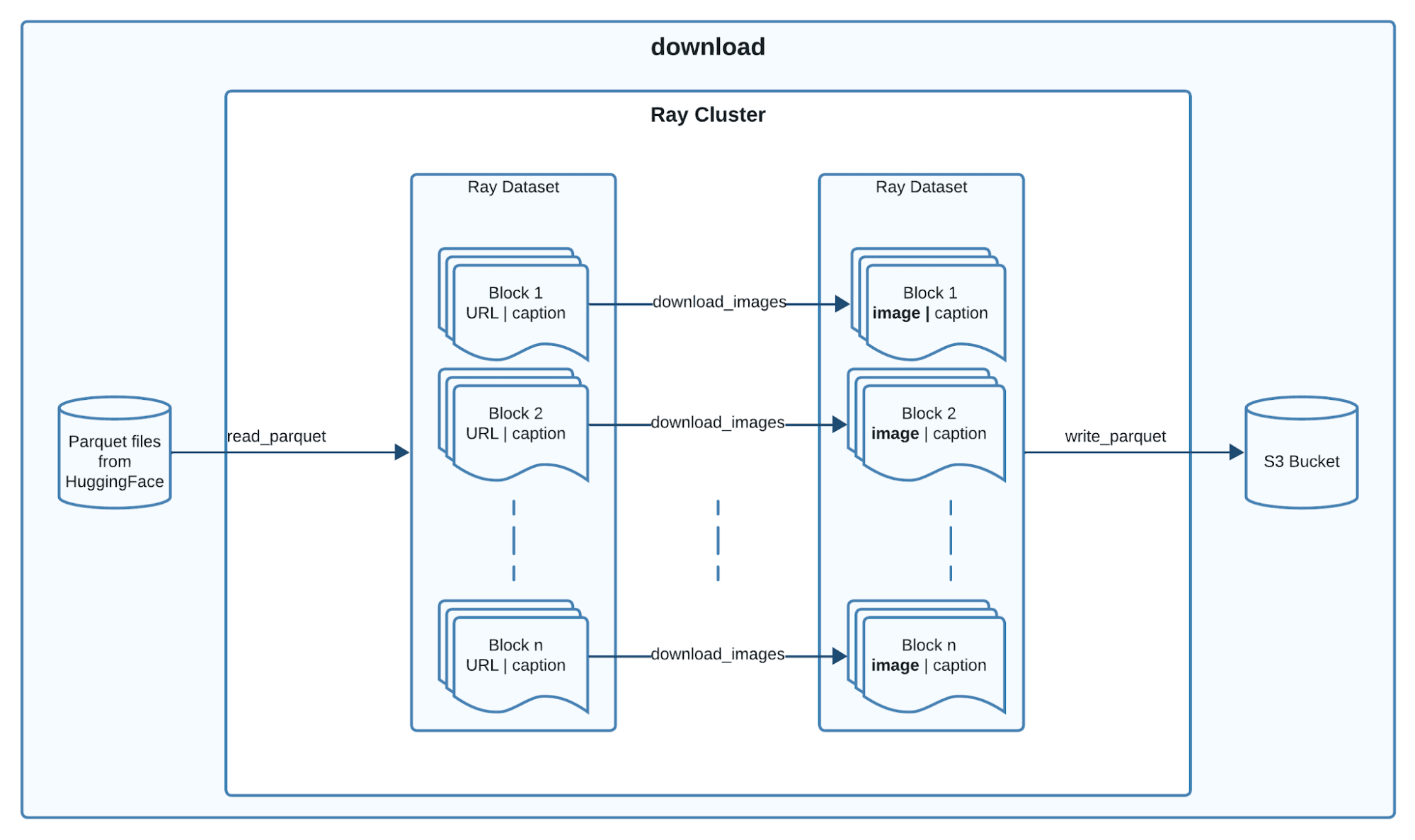Figure 4: Architecture overview of the download process.

Here is a breakdown of the above process

1. Ray Data uses Ray tasks, distributed functions, to read parquet files from hugging face in parallel.

   • Each read_parquet task reads one or more files and produces a stream of one or more output blocks.

   • The output blocks are fed directly to the downstream transform.

2. Ray Data maps the download_images transform to each output block

3. Ray Data finally writes each transformed block to the specified cloud storage in parallel. 

LinkImplementation

Link1. Reading parquet files from hugging face

The LAION Aesthetic dataset can be acquired from HuggingFace, and can be downloaded as Parquet files. Ray Data has various efficient data loaders, in particular one for Parquet files, called read_parquet.

With that in mind, let's define a get_input_dataset helper function that performs the following steps:

1. Request from the Hugging Face Hub API the URLs of the LAION Aesthetics Parquet files.

2. Load the Parquet files into a Ray Dataset using read_parquet.

1
2
3
4
5
6
7
8
9
10
11
def get_parquet_urls(path: str, name: str, split: str) -> list[str]:
    hf_api_url = f"https://huggingface.co/api/datasets/{path}/parquet"
    hf_response = requests.get(hf_api_url)
    hf_response.raise_for_status()
    parquet_urls = hf_response.json()[name][split]
    return parquet_urls

def get_input_dataset(path: str, name: str, split: str) -> ray.data.dataset.Dataset:
    parquet_urls = get_parquet_urls(path, name, split)
    ds = ray.data.read_parquet(parquet_urls, columns=["URL", "caption"])
    return ds

Note that Ray Data includes a handy from_huggingface method  for loading data from the Hugging Face Hub. However, given that Parquet is a very common format, we chose to demonstrate the read_parquet method instead. This way, you’ll be well-equipped to handle datasets from a variety of sources.

What does running the get_input_dataset helper function do?

You might be wondering whether running get_input_dataset will initiate the download of the LAION Aesthetic dataset. The answer is no. get_input_dataset calls read_parquet which in turn will only read the metadata of the Parquet files and create a Ray Dataset object that represents the data. Ray Dataset creation and transformation APIs are lazy. This means that execution is only triggered by "sink" APIs, such as consuming or writing the dataset. This is a key feature of Ray Data that allows it to handle large datasets efficiently.

A common pattern is to then apply transformations to the Ray Dataset, and finally consume it by writing the data to disk. Under the hood, Ray Data will build an execution plan that optimizes the computation and distributes it across the cluster. Optimizations include operator fusion, which combines multiple operations into a single operation to improve performance and memory stability.

Link2. Downloading the image URLs in the parquet files

Each row in the LAION parquet file contains a URL and caption as we specified in get_input_dataset. Given this URL, we can use the requests library to download the corresponding image. We do so by implementing a simple download_image function.

1
2
3
4
5
6
7
def download_image(url: str) -> bytes:
    try:
        response = requests.get(url)
        response.raise_for_status()
        return response.content
    except Exception:
        return b""

We now implement a download_images functionality that takes a batch of Parquet records and concurrently uses threads to call download_image. Some downloads might fail, e.g., due to corrupted files or wrong formatting, so we need to keep only the valid images.

1
2
3
4
5
def download_images(batch: dict[str, np.ndarray]) -> dict[str, np.ndarray]:
    with ThreadPoolExecutor() as executor:
        batch["image"] = list(executor.map(download_image, batch["URL"]))
    del batch["URL"]
    return keep_valid_images(batch)

keep_valid_images is a helper function you should implement to run validation checks for your edge cases. For example, we check if the image is non-empty with a non-negligible size and a non-empty text description.

Link3. Putting it all together into a convenient image downloading tool

With get_input_dataset and download_images utilities in place, let's write a download script that downloads the LAION Aesthetics dataset in one go. We're heavily relying on Ray Data's batch processing capabilities here, using the map_batches function to apply the download_images transform and using write_parquet to store the output.

1
2
3
4
5
6
7
8
9
10
11
12
13
14
15
16
17
18
...

@app.command()
def download(
    output_uri: str,
    dataset_path: str,
    dataset_name: str,
    dataset_split: str,
    limit: int | None = None,
    num_rows_per_output_file: int = 10000,
) -> None:
    ds = get_input_dataset(name=dataset_name, path=dataset_path, split=dataset_split)
    if limit:
        ds = ds.limit(limit)
    ds = ds.map_batches(download_images)
    ds.write_parquet(
        output_uri, try_create_dir=True, num_rows_per_file=num_rows_per_output_file
    )

To run a limited download job, you can use the following command:

1
python download.py $RAW_DATA_S3_URI laion/laion-aesthetic-120M main train --limit 1

It takes around 10 hours to download the laion-aesthetic-120M dataset without any set limit, with a total of 10 m5.8xlarge instances, which have 32 CPUs and 128 GB memory each.

Given that the data download is a one-time task where cost efficiency is prioritized over speed, we recommend using Anyscale’s spot instance support. Anyscale can handle spot instance preemptions elegantly, allowing the job to fallback onto on-demand instances to continue running smoothly.

To view the full code implementing the download script, instantly provision a Ray cluster and start running your own download,  check out the Reference Implementation on Training Stable Diffusion on Anyscale.

LinkA side note on dataset transformations in Ray Data

LinkRow vs Batch based Transformations

Transformations are applied to a Ray Data Dataset by applying one of the following methods:

• Row-based transformations

  • map: 1-to-1 operation that takes one row as an input and returns a transformed row.

  • flat_map:  1-to-n operation that takes one row as an input and returns “n” transformed row(s).

• Batch-based transformations

  • map_batches: n-to-m operation that takes one batch of size “n” as an input and returns one batch of size “m”

If your transformation can be vectorized, call map_batches for better performance.

LinkStateless vs Stateful Transformations

Transformations can either be stateless or stateful. More specifically a stateful transform is one that requires an expensive setup of a certain state. As an example of an expensive state, think of having to download model weights before being able to execute a transformation which we will see in our processing pipeline.

To avoid having to set up the state on every transformation task run, Ray Data offers the capability to spin up a pool of processes (called Actors in Ray) that load the state on creation.  Following our above example, this means Ray Data will launch a pool of processes which will already have the model weights downloaded.

Figure 5: Stateless vs Stateful transformations in Ray Data.

To define a stateful transformation in code, make use of a callable Class in python where the setup is performed in the __init__ and the transformation is performed in the __call__ method.

LinkTransforming image and text data

Let's move on to actually transforming the data we've just downloaded. What we want is a transform interface that looks like this:

1
2
3
4
5
6
7
8
9
10
11
12
13
14
15
16
17
18
19
20
21
class SDTransform:
    def __init__(self, resolution: int) -> None:
        ...

    def image_transform(self, image: bytes) -> np.ndarray:
        ...

    def tokenize(self, text: str) -> np.ndarray:
        ...

    def __call__(self, batch: dict[str, np.ndarray]) -> dict[str, np.ndarray]:
        """Transform the images and tokenize the text."""
        transformed_batch = {} 
        transformed_batch["caption_ids"] = [
            self.tokenize(caption) for caption in batch["caption"]
        ]

        transformed_batch[f"image_{self.resolution}"] = [
            self.image_transform(image) for image in batch["image"]
        ]
        return transformed_batch

In short, an SDTransform tokenizes text and transforms images suitably. We're going to define the remainder of the preprocessor’s methods in the section titled Diving deeper into the SDTransform, but assume we have them already.

LinkEncoding image and text data

After processing the data, we will need to encode the images into latents and the text into embedding vectors. What we want is an encoder interface that looks like this:

1
2
3
4
5
6
7
8
9
10
11
12
13
14
15
16
17
18
19
20
21
class SDLatentEncoder:
    def __init__(self, resolution: int, device: str) -> None:
        ...

    def encode_images(self, images: np.ndarray) -> np.ndarray:
        ...

    def encode_text(self, caption_ids: np.ndarray) -> np.ndarray:
        ...

    def __call__(self, batch: dict[str, np.ndarray]) -> dict[str, np.ndarray]:
        encoded_batch = {}
        with torch.no_grad():  
            encoded_batch[f"image_latents_{resolution}"] = (
                self.encode_images(batch[f"image_{self.resolution}"])
            )

            encoded_batch["caption_embeddings"] = (
                self.encode_text(batch["caption_ids"])
            )
        return encoded_batch

The __call__ method processes a batch of data, encoding both images and text captions into so-called latent representations. We're going to define the remainder of the encoder’s methods in the section titled Diving deeper into the SDLatentEncoder, but assume we have them already.

LinkStreaming and processing LAION data on demand

Now that we've understood how to process data in principle, let's take a bit of a leap and define the main workhorse for processing LAION data for Stable Diffusion models right away. We first give you a rundown of all steps, and then go through the relevant code snippets in detail.

The key steps are:

Step 0: Reading the raw data:

We read the raw Parquet files, which we already downloaded to S3, and load them into a Ray Dataset consisting of batches of Arrow data with our schema.

1
2
3
4
ds = ray.data.read_parquet(
    input_uri, # Raw data S3 URI
    ...
)

Step 1: Transforming the image and text data:

We apply a transform SDTransform to our dataset of images and text data.

1
2
3
4
ds = ds.map_batches(
    SDTransform,
    fn_constructor_kwargs={"resolution": resolution}  # Pass resolution to the encoder
)

Step 2: Encoding the image and text data:

Finally, we need to encode images and text, by applying the SDLatentEncoder.

1
2
3
4
5
ds = ds.map_batches(
    SDLatentEncoder,
    fn_constructor_kwargs={"resolution": resolution}, # Pass resolution to the encoder
    ...
)

The structure of the get_laion_streaming_dataset is fairly straightforward. Here's the code in full:

1
2
3
4
5
6
7
8
9
10
11
12
13
14
15
16
17
18
19
20
21
22
23
24
25
26
27
28
29
30
def get_laion_streaming_dataset(
    input_uri: str,
    batch_size: int,
    accelerator_type: str = NVIDIA_TESLA_A10G,
    limit: int | None = None,
    resolution: int = 256,
    num_encoders: int = 1,
) -> ray.data.Dataset:
    ds = ray.data.read_parquet(input_uri)
    if limit:
        ds = ds.limit(limit)

    ds = ds.map_batches(
        SDTransform, 
        fn_constructor_kwargs={"resolution": resolution},
        num_cpus=1,
        batch_size=resolution,
        concurrency=num_encoders * 2,
    )

    ds = ds.map_batches(
        SDLatentEncoder,
        fn_constructor_kwargs={"resolution": resolution},
        num_gpus=1, 
        batch_size=resolution,
        concurrency=num_encoders,
        accelerator_type=accelerator_type, 
    )

    return ds

Note that we put "stream" into the name of that function to emphasize the fact that Ray Data makes use of a streaming execution model. This means that Dataset transformations are executed in a streaming way, incrementally on the base data, instead of on all of the data at once, and overlapping the execution of operations. This can be used for streaming data loading into ML training to overlap the data preprocessing and model training.

LinkA closer look at map_batches

We take a closer look at map_batches which is the most versatile transformation method; i.e. you can think of flat_map and map as special cases of map_batches applied to a batch of size 1. 

Here is map_batches visualized in the diagram below

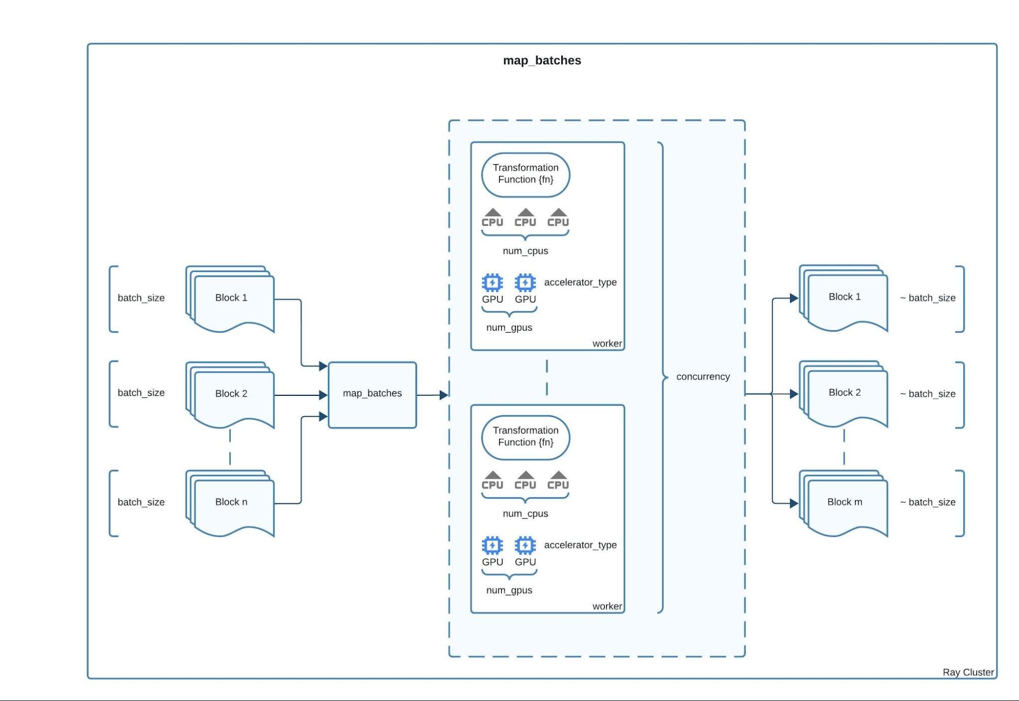Figure 6: Dataset.map_batches visualized.

Here is a detailed description of the displayed parameters:

• concurrency: control the minimum and maximum number of workers (actors or tasks)  to use.

• batch_size: The desired number of rows in each batch.

• num_gpus: the number of GPUs to reserve for each worker.

• num_cpus: the number of CPUs to reserve for each worker.

• Transformation function parameters:

  • Constructor parameters:

    • fn_constructor_args: positional arguments to pass to a callable class’s __init__ method.

    • fn_constructor_kwargs: keyword arguments to pass to a callable class’s __init__ method.

  • Call parameters:

    • fn_args: positional arguments to pass to a class’s __call__ method or a stateless transform function.

    • fn_kwargs: keyword arguments to pass to a  class’s __call__ method or a stateless transform function.

• Additional parameters like accelerator_type fall under arguments you can pass to both an actor/task. To view a complete list see the ray.remote docs page here.

For a comprehensive and up-to-date documentation of the parameters to pass map_batches, view the docs page here.

Let's now dive deeper into the transform and encoding steps needed for Stable Diffusion.

LinkDiving deeper into the SDTransform

The transformation steps for images and text data in the LAION dataset involve a few key operations.

LinkImage transformation utilities

We begin with an image transformation utility: cropping an image to its largest centered square.

Figure 7: Image before LargeCenterSquare cropping. Picture taken from unsplash.

Figure 8: Image after LargeCenterSquare cropping.

We accomplish this by implementing a LargestCenterSquare class that uses the torchvision package, which integrates seamlessly with torch and lightning, the packages we utilize during the training process.

1
2
3
4
5
6
7
8
9
10
11
12
13
14
15
16
17
18
19
20
21
22
23
class LargestCenterSquare:
    """Center crop to the largest square of a PIL image."""

    def __init__(self, size):
        self.size = size

    def __call__(self, img):
        orig_w, orig_h = img.size
        img = torchvision.transforms.functional.resize(
            img=img,
            max_size=self.size,
        )
        w, h = img.size
        c_top = (h - self.size) // 2
        c_left = (w - self.size) // 2
        img = torchvision.transforms.functional.crop(
            img=img,
            top=c_top,
            left=c_left,
            height=self.size,
            width=self.size
        )
        return img

With this utility class, we can define the SDTransform as follows:

Transform initialization:

Set all properties needed for transforming images and text - i.e. the image resolution, all image transforms needed, and the text tokenizer.

1
2
3
4
5
6
7
8
9
10
11
12
class SDTransform:

    def __init__(self, resolution: int) -> None:
        self.resolution = resolution
        normalize = transforms.Normalize((0.5, 0.5, 0.5), (0.5, 0.5, 0.5))
        self.crop = LargestCenterSquare(resolution)
        self.transforms = transforms.Compose([transforms.ToTensor(), normalize])
        self.text_tokenizer = CLIPTokenizer.from_pretrained(
            "stabilityai/stable-diffusion-2-base", subfolder="tokenizer"
        )

    ...

Image transform:

First, we ensure the image is in RGB format, then we apply LargestCenterSquare to crop the image, and finally we normalize all RGB channels with the transforms callable.

1
2
3
4
5
6
7
class SDTransform:
    ...

    def image_transform(self, image: bytes) -> np.ndarray:
        image = self.ensure_rgb(image)
        image = self.crop(image)
        return self.transforms(image)

Text tokenization:

Text tokenization is a transformation step that converts text into a list of tokens, which are then converted into numerical values for the model to process.

Below is text tokenization visualized for a single caption:

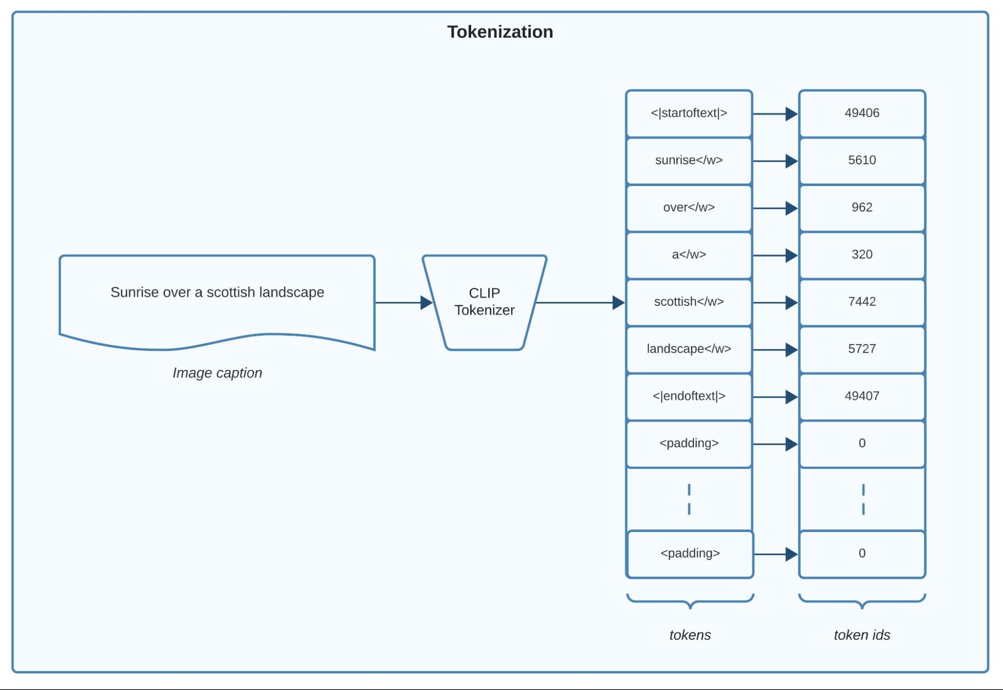Figure 9: CLIP Text tokenization. 

We use the tokenizer from a pretrained CLIP model, available through the transformers library. CLIP models embed text and images simultaneously, ensuring the embeddings are closely related.

1
2
3
4
5
6
7
8
9
10
class SDTransform:
    ...

    def tokenize(self, text: str) -> np.ndarray:
        caption_ids = self.text_tokenizer(
            text,
            ...
        )["input_ids"][0]

        return caption_ids

To view the full code implementing SDTransform,  check out the Reference Implementation on Training Stable Diffusion on Anyscale.

LinkDiving deeper into the SDLatentEncoder 

Now, let's examine the details of the SD encoder for both images and text. 

SDLatentEncoder Initialization

The SDLatentEncoder class initializes with the device and resolution parameters. It loads the VAE and CLIP models from the "stabilityai/stable-diffusion-2-base" model on the Hugging Face model hub. The VAE model encodes images, while the CLIP model encodes text.

1
2
3
4
5
6
7
8
9
10
11
12
13
14
15
16
17
18
19
20
21
22
class SDLatentEncoder:

    def __init__(
        self,
        resolution: int = 256,
        device: str = "cuda",
    ) -> None:
        self.resolution = resolution
        self.device = device

        self.vae = AutoencoderKL.from_pretrained(
            "stabilityai/stable-diffusion-2-base",
            subfolder="vae", 
        )

        self.text_encoder = CLIPTextModel.from_pretrained(
            "stabilityai/stable-diffusion-2-base",
            subfolder="text_encoder",
            torch_dtype=torch.float16,
        )

        ...

Step 1: Encoding Images

Images are encoded into a latent distribution using a Variational Auto-Encoder (VAE) model. The latent samples are scaled and converted to an array, then added to the batch.

We visualize a variational autoencoder below:

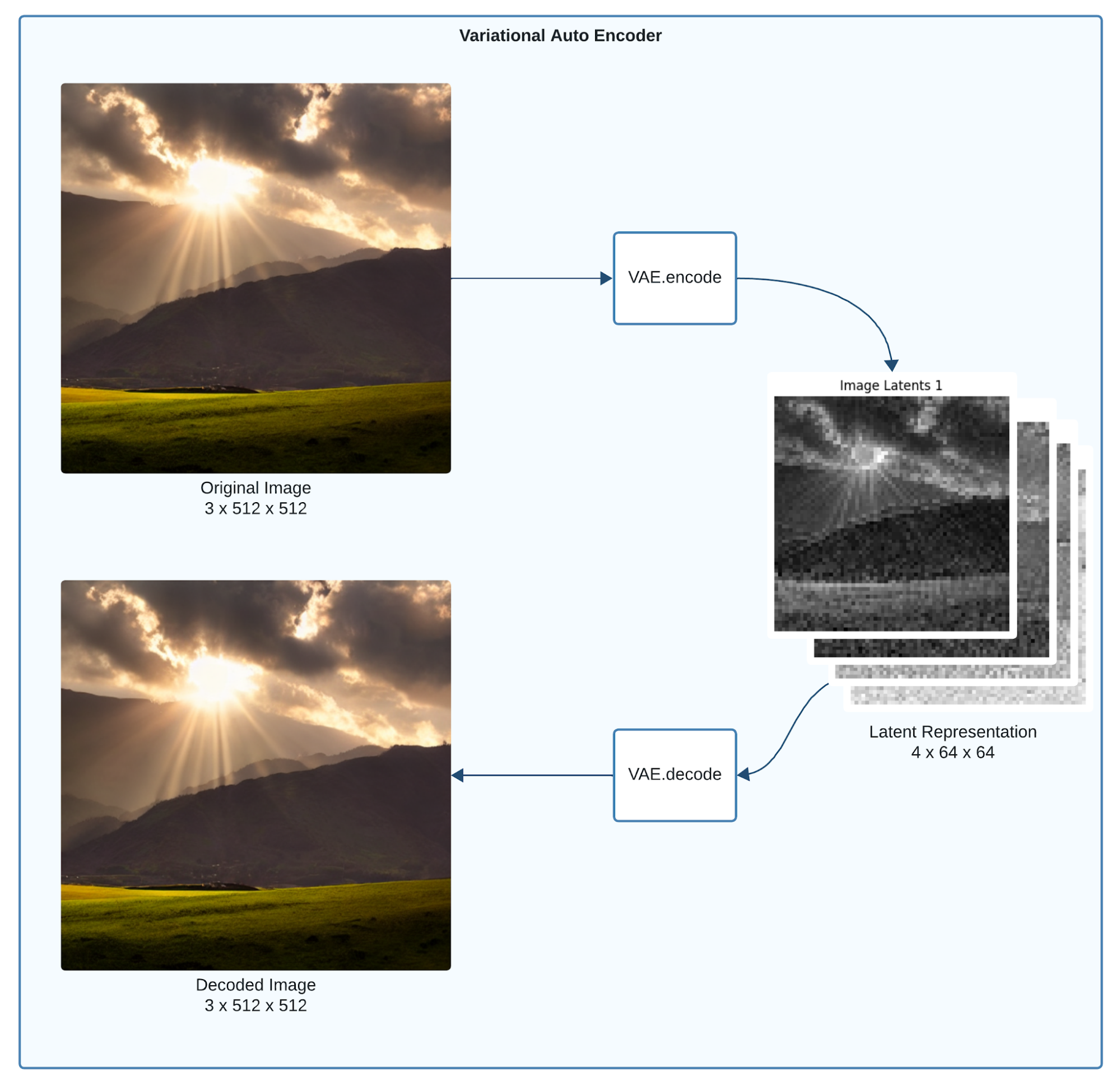Figure 10: Variational Autoencoder with a sample input, representation and output.

Note the diagram depicts the decoder step, which we currently don't need yet, but will become important later on when we want to generate images. In that case, the latent representations have to be converted back to images that make sense to humans.

Here is how the SDLatentEncoder.encode_images method can be implemented:

1
2
3
4
5
6
7
8
9
10
11
12
13
class SDLatentEncoder:
    ...

    def encode_images(self, images: np.ndarray) -> np.ndarray:
        input_images = torch.as_tensor(
            images,
            device=self.device,
            dtype=torch.float16
        )
        latent_dist = self.vae.encode(input_images)["latent_dist"]
        unit_variance_scaling_factor = 0.18215
        image_latents = latent_dist.sample() * unit_variance_scaling_factor
        return image_latents.detach().cpu().numpy().astype(np.float32)

Step 2: Encoding Captions

Caption ids are encoded using the text encoder model. The caption embeddings are converted to an array and added to the batch.

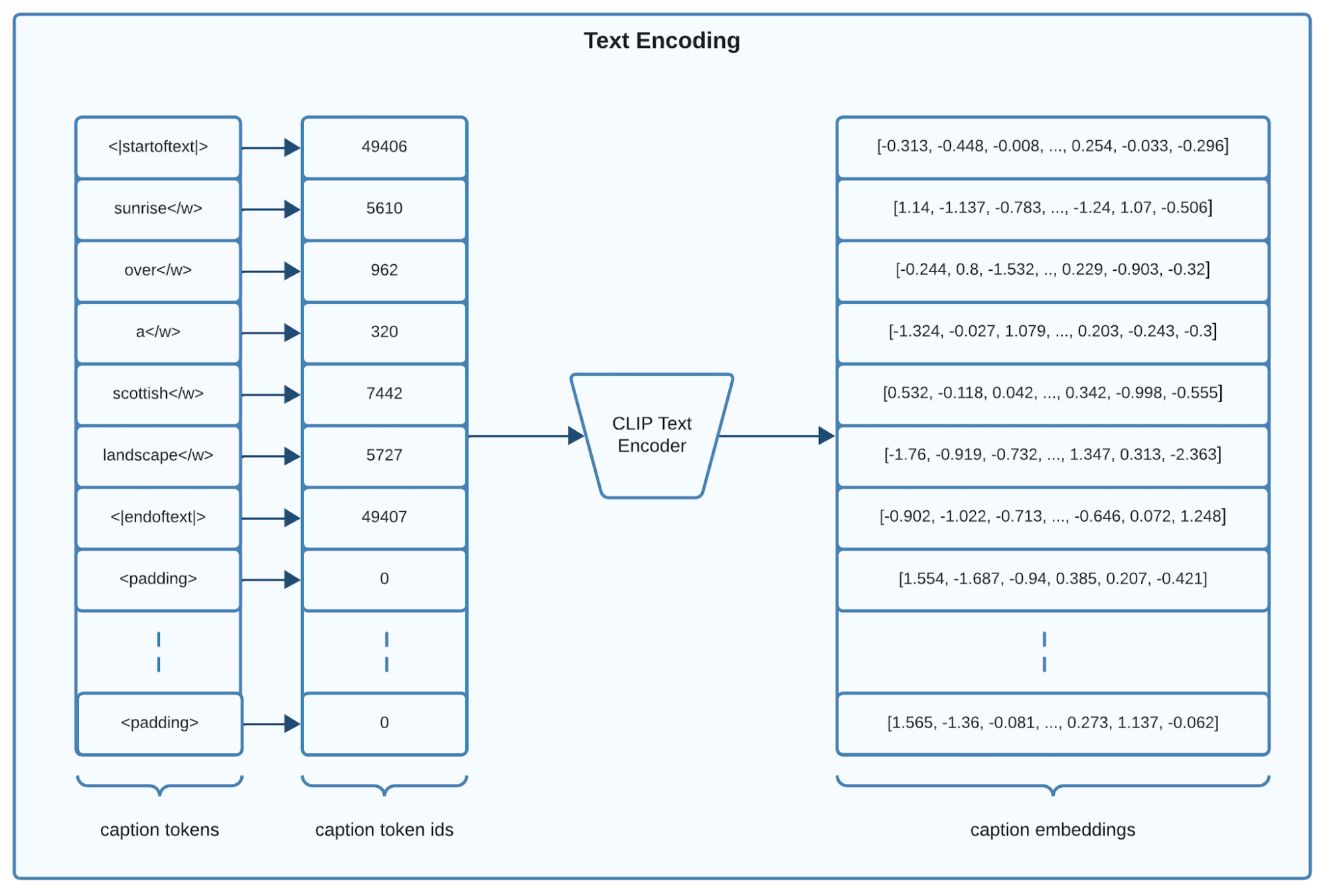Figure 11: CLIP model’s text input and output. 

Here is how the SDLatentEncoder.encode_text method can be implemented:

1
2
3
4
5
6
7
class SDLatentEncoder:
    ...

    def encode_text(self, caption_ids: np.ndarray) -> np.ndarray:
        caption_ids_tensor = torch.as_tensor(caption_ids, device=self.device)
        caption_embeddings_tensor = self.text_encoder(caption_ids_tensor)[0]
        return caption_embeddings_tensor.detach().cpu().numpy().astype(np.float32)

To view the full code implementing SDLatentEncoder and start running your own data processing,  check out the Reference Implementation on Training Stable Diffusion on Anyscale.

LinkPutting it all together into a performant processing script

We have completed the necessary steps to process the LAION Aesthetics dataset for training. Let's encapsulate these steps into a script that processes the raw LAION data stored on S3.

Note how get_laion_streaming_dataset does all of the work, the rest of the process function below is mostly scaffolding to allow for parametrization and writing out the processed data.

1
2
3
4
5
6
7
8
9
10
11
12
13
14
15
16
17
18
19
20
21
22
23
24
25
26
27
28
29
30
import typer

app = typer.Typer()

...

@app.command()
def process(
    raw_data_uri: str = typer.Argument(..., help="The input URI for raw data."),
    output_uri: str = typer.Argument(..., help="The output URI for the processed data."),
    batch_size: int = typer.Option(None, help="The batch size to use.")
    accelerator_type: str = typer.Option("NVIDIA_TESLA_A10G", help="Accelerator type."),
    resolution: int = typer.Option(512, help="The resolution for image processing."),
    num_rows_per_output_file: int = typer.Option(5000, help="Number of output rows."),
    num_encoders: int = typer.Option(1, help="The number of encoder workers to use."),
    limit: int = typer.Option(None, help="The number of rows to process."),
):
    ds = get_laion_streaming_dataset(
        input_uri=raw_data_uri,
        resolution=resolution,
        batch_size=batch_size or get_default_batch_size(resolution),
        num_encoders=num_encoders,
        accelerator_type=getattr(ray.utils.accelerators, accelerator_type),
        limit=limit,
    )

    ds.write_parquet(output_uri, num_rows_per_file=num_rows_per_output_file)

if __name__ == "__main__":
    app()

Execute the processing script on a cluster with the following command:

1
python process.py $RAW_DATA_S3_URI $PROCESSED_DATA_S3_URI --resolution 256

Note that to scale you will need to provision a cluster with multiple A10 GPUs. To view the full code implementing process.py and easily provision the infrastructure to start running your own data processing,  check out the Reference Implementation on Training Stable Diffusion on Anyscale.

LinkOptimizing Your Processing Pipeline For Cost and Performance

Tuning your processing pipeline involves balancing performance with cost, especially under budget constraints. You can fine-tune our pipeline by adjusting the following components:

• Number of GPUs: Increase the number of GPUs to speed up the encoding of images and text.

• Accelerator Type: Select the appropriate instance type for running GPU-based encoding tasks.

• Batch Size: Modify the batch size to effectively balance memory usage and processing speed.

• Number of CPUs: Increase the number of CPUs to enhance task parallelism and throughput.

LinkKey Metrics to Monitor

• GPU Memory Usage and Utilization: Ensuring high memory usage and utilization indicates that the GPU is not bottlenecked by upstream processing issues, and that data is being fed in at the appropriate batch size.

• CPU Memory Usage and Utilization: Adjust the number of CPUs to optimize parallel processing. Employing too many CPU workers can lead to increased communication overhead and underutilization of processing nodes.

The primary goal of these adjustments is to improve the pipeline's efficiency—specifically, reducing preprocessing times for datasets such as the LAION dataset, while maintaining favorable cost-scaling properties.

To optimize performance for your dataset size and chosen parameters, it's important to understand the scaling attributes. For insights into the tuning process, we recommend reading Scalable and Cost-Efficient Stable Diffusion Pre-training with Ray. This resource provides valuable guidance on adjusting your setup for maximum efficiency.

LinkMonitoring metrics using the Ray Dashboard

Using the Ray Dashboard, you can monitor the performance of the processing pipeline and identify bottlenecks. The Ray Dashboard provides real-time hardware utilization metrics as shown in the screenshot below:

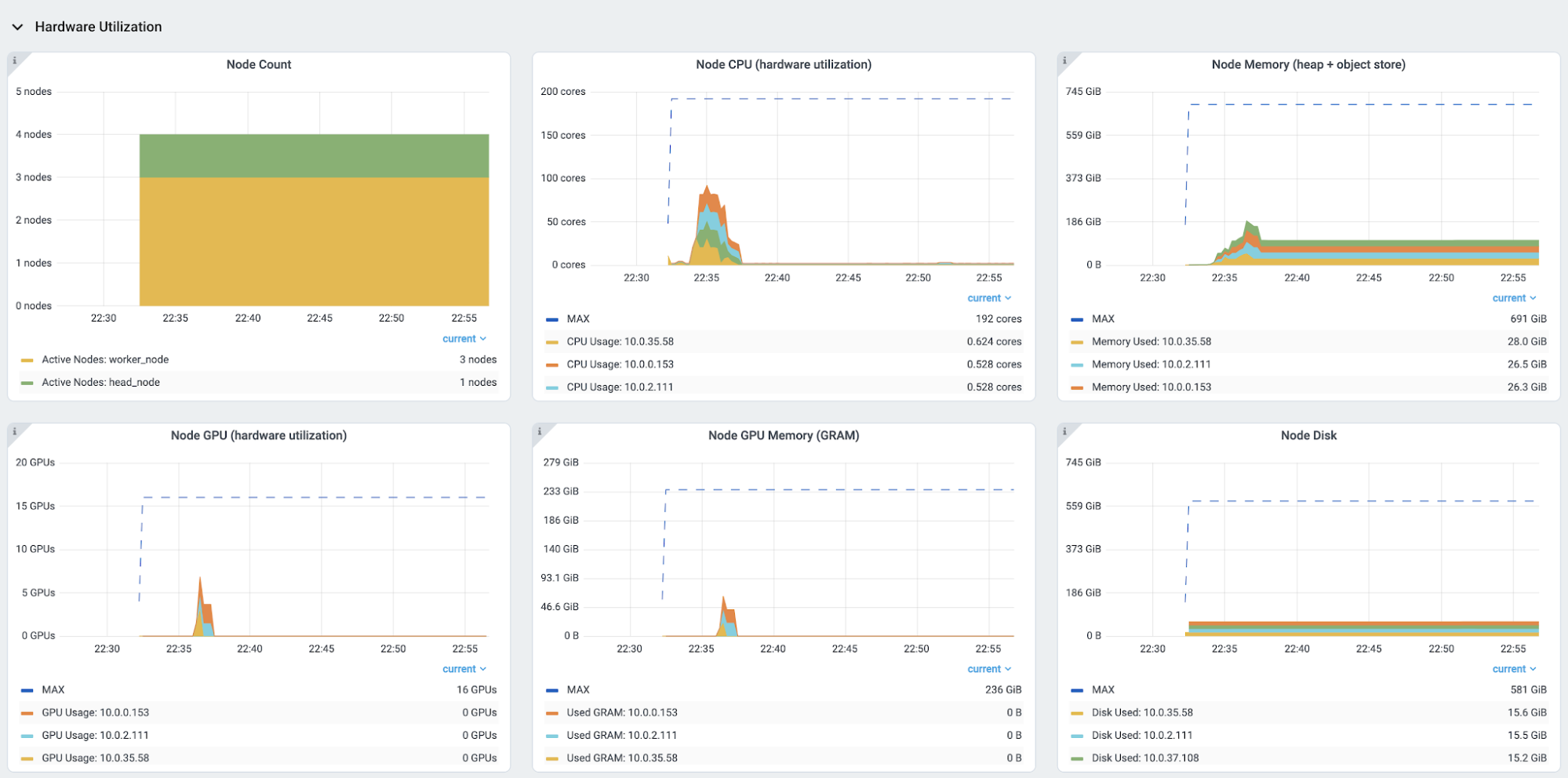Figure 12: Ray Dashboard partial screenshot of the Metrics tab’s Hardware Utilization section.

Please note that for an enhanced Ray Dashboard experience—which includes features like viewing time-series metrics alongside logs, job information, and more—you will need to set up Prometheus and Grafana and integrate them with the Ray Dashboard. Dashboards are built into Anyscale and available by default.

LinkKey Takeaways

In this guide, we've learned how to develop an end-to-end data processing pipeline for training Stable Diffusion models at scale. More specifically, we have learned the following:

• How to download and process the LAION Aesthetics dataset using Ray Data enabling us to directly stream the data from huggingface hub to S3.

• What the image and text transformation steps are that are needed for training Stable Diffusion models, and we've seen how to scale these transformations using Ray Data

• How to encode images and text data as inputs for our main Stable Diffusion model and how to leverage GPUs to speed up these computations.

• How to tune a data pipeline for performance and cost efficiency.

To view the full code implementing both the download and process scripts, instantly provision a Ray cluster and start running your own Stable diffusion data processing, check out the Reference Implementation on Training Stable Diffusion on Anyscale.

LinkFuture Work

In future guides, we aim to show the code for training more recent versions of Stable Diffusion models (such as Stable Diffusion XL or Stable Diffusion V3) which entail even more challenging resource requirements and data processing requirements.

LinkConclusion

Overall, having image data streamed across a heterogeneous cluster of CPUs and GPUs into ML models is where Ray shines as a scalable solution offering clear improvements in cost and performance.

To proceed with pre-training your Stable diffusion model, check out Definitive Guides with Ray on Pre-Training Stable Diffusion Models on 2 billion Images Without Breaking the Bank.

If you are impatient and want to run our reference implementation right away, check out this pre-packaged solution with all the code.