Shuffle V2 in Ray Data: Faster, Fault-Tolerant Joins and Aggregations

Whether the output is a training corpus, a batch of model predictions, or an evaluation report, the same operations keep appearing: deduplicating billions of records, joining features, modalities, or model outputs across sources, and computing per-group statistics to filter, sample, and score. Each of those is a shuffle.

Shuffle is the one operation Ray Data cannot stream. A map or a write takes a block, transforms it, and passes it downstream, so peak memory tracks block size rather than dataset size. groupby, join, and repartition require every row sharing a key to be gathered in one place, so a shuffle worker holds a partition, and partition size is the dataset divided by the partition count. Ten times the data means ten times the memory in that worker.

Shuffle is where these pipelines fail, where the OOMs happen, and where a job that ran fine at 100 GB falls over at 1 TB.

Shuffle V2 is a redesign of Ray Data's shuffle engine. It materializes shuffle intermediates in the object store instead of accumulating them in a long-lived aggregator, which gives us:

• Stability: shards live in the object store, spilled to disk when it fills, so intermediates no longer pile up in a worker's heap.

• Scalability: map and reduce are ordinary tasks, so Ray runs as many at a time as the cluster has room for, instead of a number picked before any data arrives.

• Efficiency: the decoupled design admits optimizations the old engine could not express: vectorized aggregation, fusion across the shuffle boundary, and compression.

LinkWhere V1 breaks down

The current Ray Data shuffle leverages a pool of long-lived aggregator actors. Map tasks partition their blocks and submit each shard to the actor that owns that partition. The actor holds those shards until the shuffle completes, then finalizes each partition into output blocks.

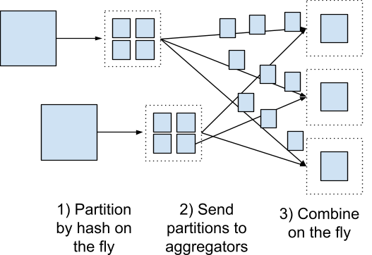
The current design has a critical property - that partition state accumulates in a long-lived actor's heap. However, this results in a variety of issues.

1. A dataset cannot be larger than memory
Every shard belonging to a partition sits in its aggregator's heap until the shuffle completes, so at peak the cluster has to hold the whole dataset in actor heaps at once.

How much that costs depends on the operation. Reducing aggregations — sum, count, unique — can compact partial shards as they arrive, folding them into a running result, so their state is bounded by the number of distinct groups rather than by the dataset. Concatenating operations cannot. A join or a key-based repartition has to keep every row it has received and combine only at finalization, so the aggregator ends up holding the entire partition.

2. Lost state cannot be rebuilt
A partition exists only inside the actor accumulating it, and there is no lineage-tracked copy anywhere else for Ray to rebuild it from. Losing one aggregator loses every partition it owned, and the shuffle cannot recover.

3. The aggregator pool is sized once, from an estimate
The pool is sized from a sample of the first few input bundles, long before most of the data has been seen. A skewed dataset or unrepresentative samples leave a pool that is wrong for what actually arrives, and there is no way to resize it once the shuffle has started.

4. Reservations are held for the entire shuffle
Aggregators are reserved up front, so num_aggregators x num_cpus is held from the moment the pool starts until the last partition is finalized, whether or not those actors are doing work. This leaves only a small amount of resources for other operators to use.

LinkArchitecture

V2 splits the shuffle into two ordinary stages with the object store between them.

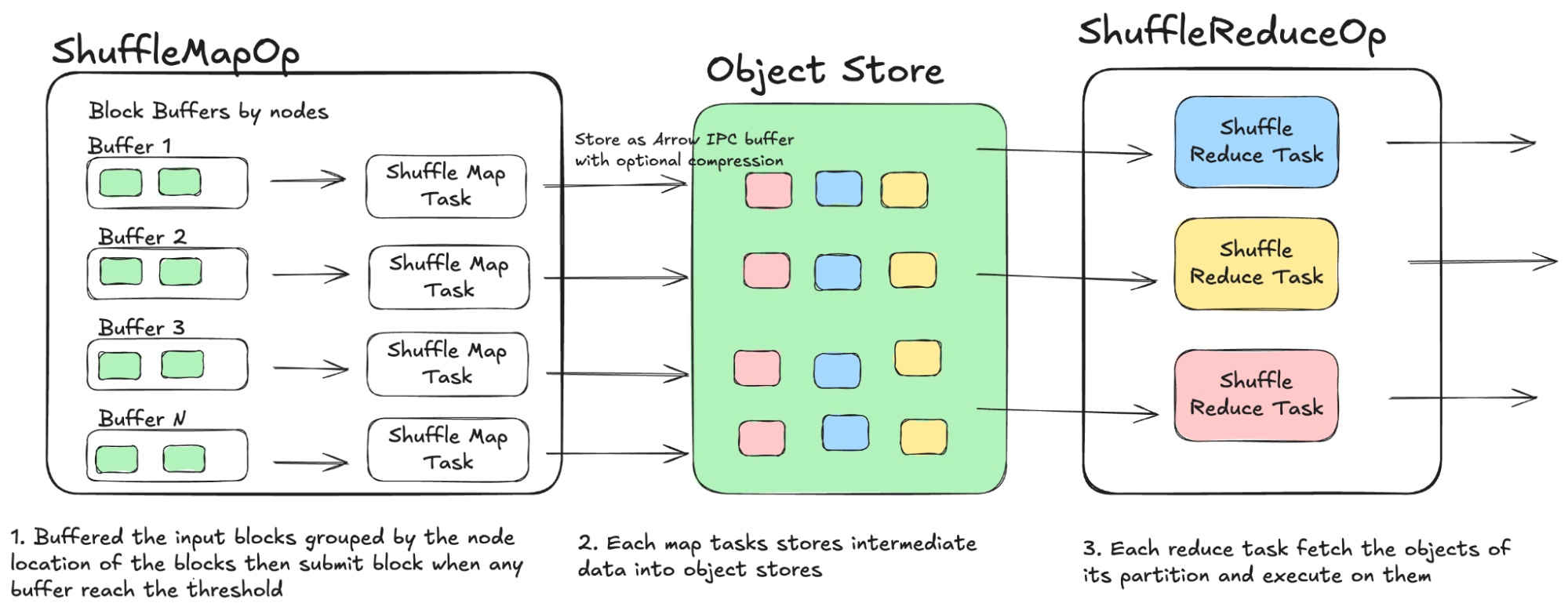
The map stage partitions each input block by key and returns one shard per partition, num_partitions + 1 values per task, one for metadata and one for each partition. Each shard is encoded as an Arrow IPC buffer, optionally compressed, and lands in the object store as its own object with its own reference.

The reduce stage assigns one partition per task. A reduce task receives the shard references for its partition, pulls them in batches, decodes them, and applies the aggregation. Nothing is pushed into it; it fetches what it needs when it is ready.

That one change, intermediates living in the object store rather than in an actor's heap, solves each of V1's problems in turn.

1. Spilling replaces the memory ceiling
Shards are object-store objects, and the object store spills to disk under pressure, so shuffle intermediates are no longer capped by RAM. 

2. Leveraging Ray Core’s lineage reconstruction 
Because shards are ordinary Ray objects. A lost shard is rebuilt by re-executing the map task that produced it. Consequently, losing any individual shard will not cause the entire job to fail.

3. Reducer memory comes from measurement
Instead of relying on pre-shuffle estimations to size reducer actors, we directly measure partition shards to determine their actual size, this mitigates reducer OOM errors caused by inaccurate estimates.

4. No stage holds resources another stage needs
There is no aggregator pool, so nothing reserves CPU for the duration of the shuffle. Map and reduce acquire resources when they are scheduled and hand them back when they finish, so capacity flows to whichever stage actually has work, the upstream read, the map stage, or a reduce task, instead of sitting idle inside actors waiting for shards to arrive.

LinkWhat V2 unlocks

A materialized boundary between two ordinary stages is not just safer, but also easier to optimize. Each of the following is something the aggregator design could not express.

LinkInput coalescing

Every map task emits one shard per partition, so the shuffle produces map_tasks x partitions intermediate objects. With one map task per input block, that number grows with the input block count and quickly reaches a point where the head node is unable to manage all these objects and OOMs.

Coalescing shrinks the first of those two factors, the number of map tasks. Blocks are buffered and merged into a single map task once the buffer reaches shuffle_input_batch_bytes, 1 GiB by default, so fewer and larger map tasks emit proportionally fewer shards without changing how much data moves. Buffering is keyed by node, so a coalesced task also runs where its inputs already are, which prevents additional object transfer.

LinkCompression of intermediate shards

Shards are Arrow IPC buffers, and the IPC write options carry a codec, zstd by default, with lz4 and none available through hash_shuffle_compression. This helps us cut down the data size of intermediate objects, saving space and improving object transferring performance.

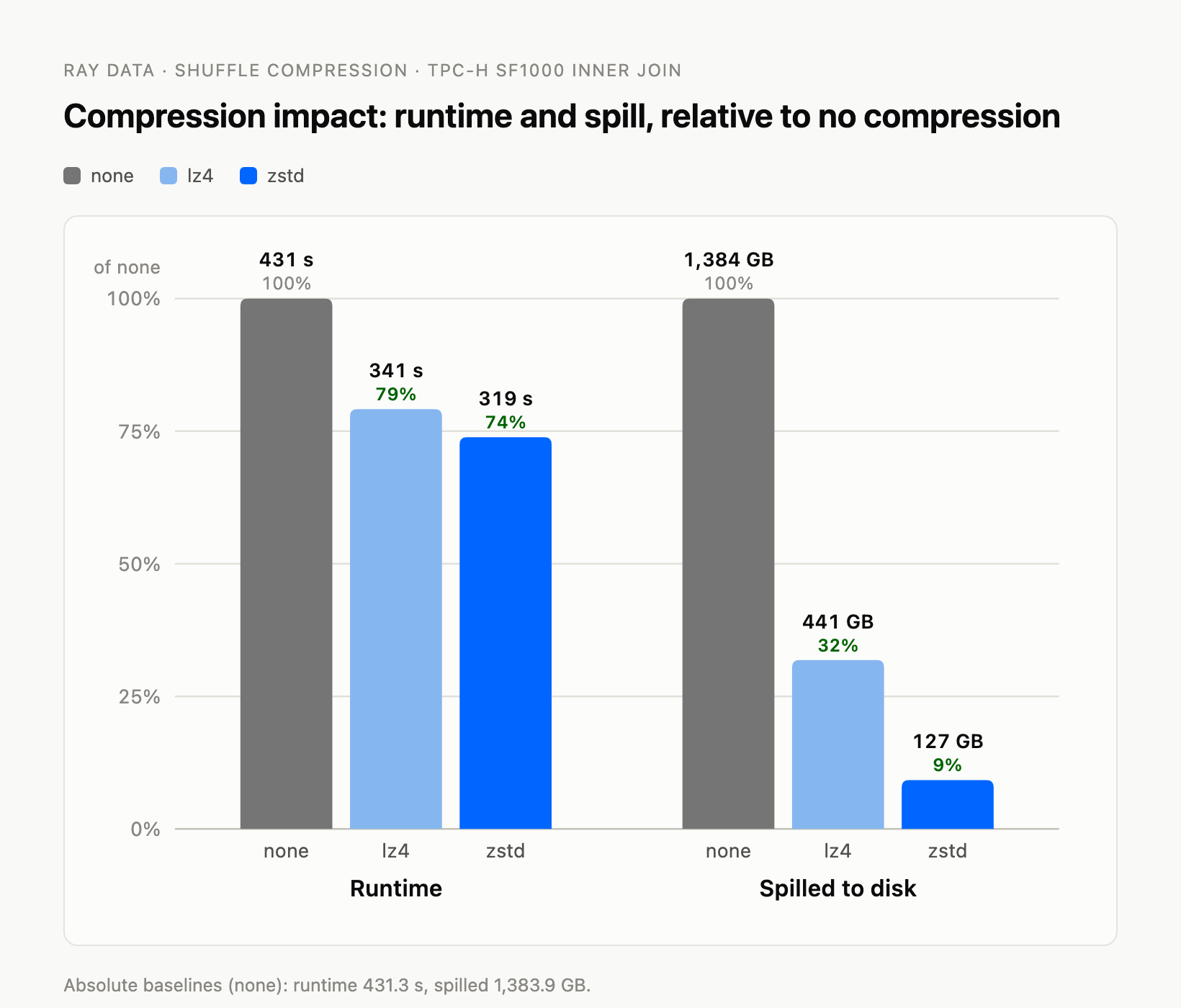
To show what compression buys, we ran the SF1000 join benchmark on 1 m5.2xlarge head node and 32 m5.4xlarge workers, on Ray 2.58. zstd compresses harder at a higher CPU cost; lz4 compresses less for far less CPU.

Compared with no compression, zstd cuts spilled bytes by 91% and runtime by 26%. lz4 spills more than zstd but still cuts spilled bytes by 68% and runtime by 21%. The extra CPU zstd spends is more than repaid by the bytes it keeps out of the spill path. 

Which codec to use depends on where the job is bottlenecked: zstd trades CPU for fewer bytes, lz4 does the opposite. Pick zstd when the shuffle is IO-bound, lz4 when it is CPU-bound and none when the data is already compressed.

LinkFusion across the shuffle boundary

A map immediately downstream of the reduce is folded into the reduce task itself. A groupby().sum() followed by map_batches() no longer writes the aggregation result out and reads it back; the map runs inside the reduce task against blocks already in memory, and one materialization disappears.

Only that side of the boundary fuses today. An upstream map cannot yet be folded into the map stage, because coalescing buffers blocks across bundles before deciding what a map task will process, and there is no single upstream task to fuse into at the point the decision is made. Reconciling the two, keeping the lower object count while still absorbing the upstream map, is work we intend to take on.

LinkVectorized aggregations

V1 aggregated by iterating group by group in Python and accumulating a result per group. V2 hands the whole block to Arrow's native group-by instead, on both the map and the reduce side, so the aggregation runs as a single columnar operation over the entire block rather than a loop over groups.

Nine aggregations are vectorized today: Count, Sum, Min, Max, Mean, MissingValuePercentage, ZeroPercentage, Unique, and CountDistinct.

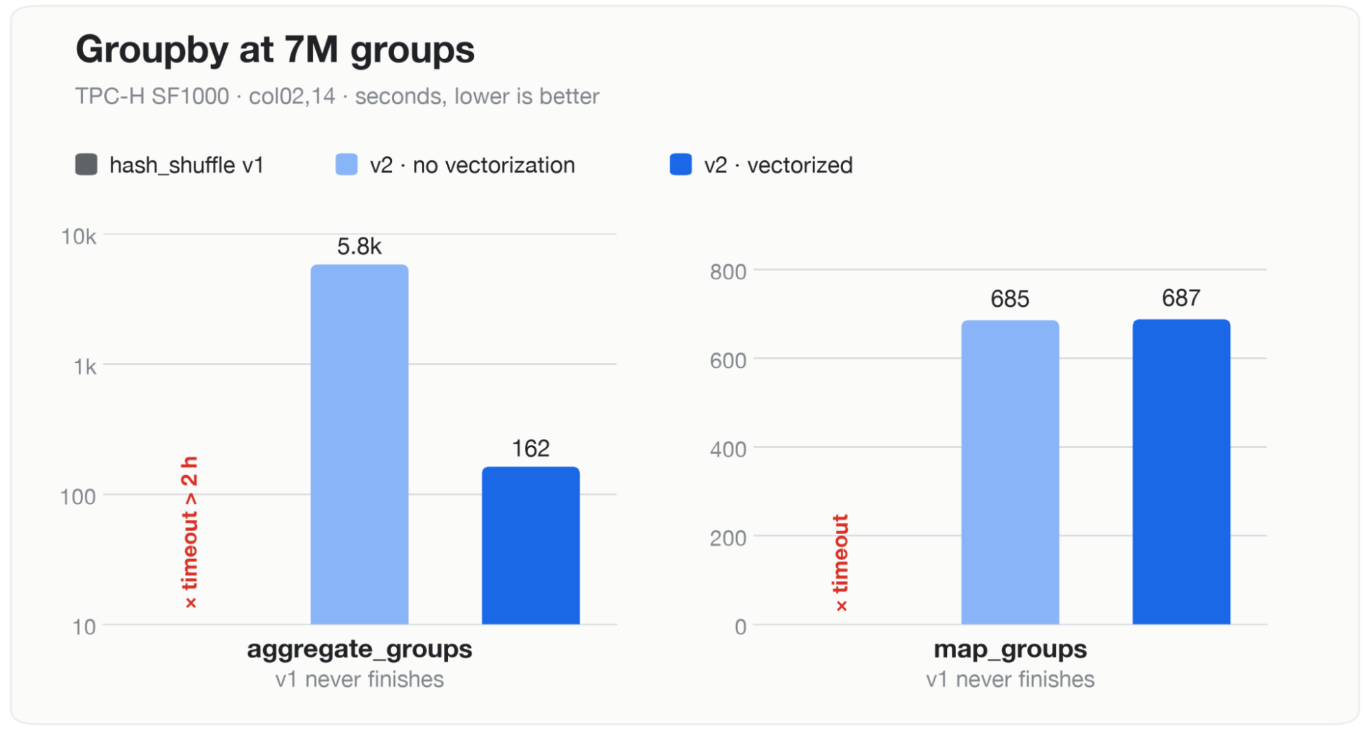
This alone gives us more than 30x performance improvement on aggregate_groups tests.

LinkDisk shuffle

Input coalescing reduces the number of intermediate objects, but it does not remove the ceiling. The driver still holds a reference to every shard, and there is a hard limit on how many it can track. The count costs throughput at both ends as well: map tasks putting many small objects into the object store, and reduce tasks dereferencing many of them at once, are both slower than moving the same bytes in bulk.

To push the boundary further, disk shuffle takes the object store out of the data path altogether. Three changes make that work.

1. Intermediate data bypasses the object store

Map output goes straight to local disk instead of into plasma, so shuffle data never occupies object-store memory and never pays for a spill.

2. One file per mapper, indexed by offset

A mapper writes a single file and returns a handle holding its path and a per-partition index of (offset, length) pairs. The map_tasks x partitions object count collapses to one handle per mapper, and a reduce task reads its partition as a byte range out of each file.

3. An Arrow Flight server on every node

Each node runs a detached actor that serves partition ranges over Arrow Flight, so shards travel as Arrow record batches on a protocol built for moving columnar data rather than a wire format of our own. One file server per node serves all reads; reducers batch byte ranges over a single Flight connection per node, and the server fetches each range via seek + read in request order.

We aim to release disk shuffle in 2.59.

LinkBenchmarks

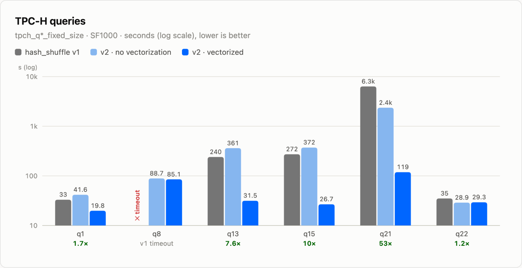
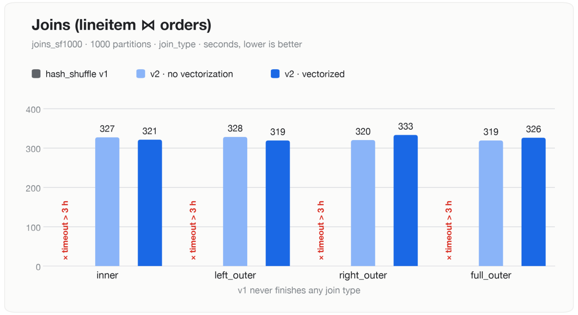
All numbers below come from Ray Data's release test suite on TPC-H data, at SF1000 using a cluster with 1 m5.2xlarge head node and 32 m5.4xlarge worker nodes running Ray 2.58. Every configuration was given identical resources, and each chart reports three of them: V1 hash shuffle, V2 with vectorized aggregation disabled, and V2 as it ships. Every run also lowers Ray's inline threshold to RAY_max_direct_call_object_size=8192, to keep small shards from being sent inline through the driver, which can OOM it (see tuning guide for more info on this configuration); the one exception is the V1 join configuration, which uses the 100 KiB default. The middle bar exists to separate what the architecture contributes from what vectorization contributes, and the two turn out to matter for different workloads.

Bars marked timeout did not finish. Their speedup figures are lower bounds computed against the timeout, so the real gap is larger than the number shown.

Two effects account for nearly all of the difference, and which one dominates depends on the workload.

Where aggregation dominates, vectorization wins. TPC-H q21 and the aggregate_groups cases spend most of their time in the aggregation combiner, and handing that work to Arrow's native groupby is worth another 20x on top — q21 goes from 6.3k seconds to 2.4k on the architecture alone, and to 119 seconds once vectorization lands, 53x end to end. The middle bar also shows where the architecture loses on its own: q1, q13 and q15 come out slower than V1 (361s against 240s, 372s against 272s). That happens when little data really gets shuffled — a filter or projection upstream leaves the shuffle small, so V2's extra encode and object-store round trip cost more than the architecture saves. Once vectorization kicks in, V2 wins every query.

Where V1 does not finish at all, the architecture wins. Joins and map_groups run no aggregation combiner, so vectorization has nothing to act on and the architecture is all that is left. At this data size V1's aggregator pool holds its CPU reservation for the entire shuffle, leaving the map phase to compete for what is left. V2 has no pool to reserve: map and reduce take resources when they are scheduled and hand them back when they finish, so capacity flows to whichever stage has work. All four join types complete in about 320 seconds.

LinkEnabling it

Starting from Ray 2.58 you can enable shuffle V2 via: 

from ray.data.context import DataContext, ShuffleStrategy

DataContext.get_current().shuffle_strategy = ShuffleStrategy.HASH_SHUFFLE_V2

The upcoming Ray 2.59 renames this strategy to SHUFFLE_V2, since it is no longer specific to hash partitioning. HASH_SHUFFLE_V2 remains as an alias, so the snippet above keeps working.

See tuning guide to learn more about the details.

LinkThe shuffle strategy landscape

Turning V2 on means setting a shuffle strategy, and Ray Data currently exposes

five: HASH_SHUFFLE (V1, and today's default), HASH_SHUFFLE_V2, GPU_SHUFFLE, SORT_SHUFFLE_PULL_BASED, and SORT_SHUFFLE_PUSH_BASED.

As V2 grows to cover the operators still served by the sort-based engines, those strategies and V1 will soon be deprecated, leaving SHUFFLE_V2 and GPU_SHUFFLE as the only two that remain.

LinkWhat's next

LinkSort and random_shuffle on V2

sort() and random_shuffle() still run on the sort-based engines. Moving them onto V2's materialized shards is what lets those strategies be retired.

LinkIncremental join

A join today materializes both sides of its partition and then the entire output table alongside them. Building a hash table from one side and streaming the other through it in batches would bound that to the build side plus one batch. This depends on Arrow 26.0.0; we will support it once that release lands.

LinkTry it out now!

Shuffle V2 comes down to one decision: shuffle intermediates live in the object store instead of a long-lived actor's heap. Everything else follows from that. Spillable, lineage-tracked shards are why joins and map_groups that V1 could not finish are now complete, and two ordinary stages with a materialized boundary between them are what let coalescing, compression, fusion, and Arrow-native aggregation land on top.

If your pipelines groupby, join, or repartition by key at any real scale, V2 is worth turning on today. Stay tuned and refer to the guides and internals for more details!