Time Series Forecasting using an LSTM version of RNN with PyTorch Forecasting and Torch Lightning

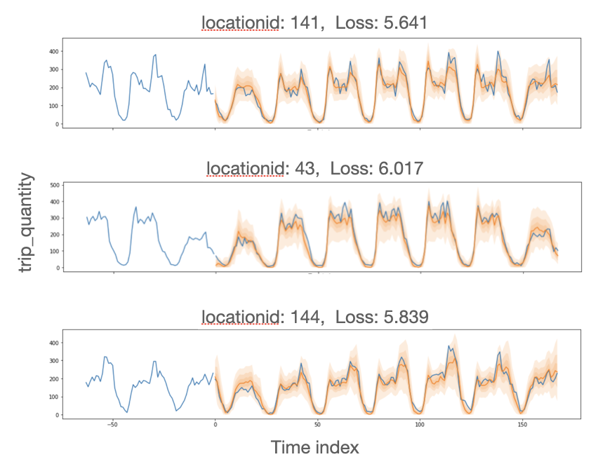Displaying New York City Yellow Taxi ride volumes, with 1 week hourly forecast. Blue=observed, Orange=predicted, per validation dataset. Forecast generated using Google’s Temporal Fusion Transformer algorithm implemented by Pytorch forecasting, and parallelized by Ray for faster runtime, either on a laptop or on any cloud. Image by Author.

In Part 1, my previous blog explained how to apply the “Embarrassingly Parallel” pattern to speed up forecasting when each model is independently trained, such as with traditional forecasting algorithms ARIMA, Prophet, and Neural Prophet. Data, Training and inference get distributed by the Ray engine across local laptop cores. The concept is similar to Multiprocessing Pool, except Ray can handle distributing more complex classes and functions. Unlike Multiprocessing, the exact same code can run in parallel across any cluster in any cloud too.

This post will explain how to use Ray to speed up Deep Learning forecasting when training one large global model in order to predict many target time series. Why do this? Well, often, things a company wants to forecast are related to each other like sports fan items, washer and dryer that are the same brand and color, supermarket items that are often bought together, etc. Then each target time series is used as input to the same model, and each gets a different output.

Parallelizing code for distributed runtime of global deep learning models requires Distributed Data Parallelism and Model Parallelism. This requires co-ordination between distributed compute nodes to shard the data, share the gradients between nodes each with its own data shard, and combine the gradients into a single global model. Ray handles the Data and Model Parallelism, while keeping a simple API for developers. Further, Ray can train and inference the Deep Learning model in parallel, distributed across a single laptop’s cores or across compute nodes in any cloud.

This blog is organized into the following topics:

• Intro Deep Learning AI algorithms used in forecasting

• Using Google’s Temporal Fusion Transformer in Pytorch Forecasting (uses PyTorch Lightning APIs)

• How to speed up model training and inference using Ray

• How to speed up model training and inference in any cloud using Anyscale 

LinkIntro Deep Learning AI Algorithms used in Forecasting

Left. High-level view of an RNN and unfolded time steps. Image source.
Middle. Typical ANN building block, consisting of 1 input layer, 2 hidden dense layers, and an output layer. Image source. Right. Example GRN consisting of 2 dense layers, with 2 activation functions (ELU exponential linear unit and GLU gated linear unit), and dropout. Image from Temporal Fusion Transformer paper.

A Recurrent Neural Network ( RNN) is a type of neural network that is often used for time series since it processes data sequentially. RNN consists of a sequence of ANNs (artificial neural network) per fixed time step. Each ANN building block is a set of neurons divided into input layer, hidden layers and output layer, where each neuron is connected to other neurons and each connection has a trainable weight. RNNs were first used for text translation.

Following are some related concept terms.

LSTM (Long Short-Term Memory) is a type of recurrent neural network architecture, designed to overcome the vanishing gradient problem (where things way in the past might get close to 0-value weights). LSTM has 3 memory gates which together allows a network to remember and forget.

GRN or Gated Residual Network can replace a basic ANN building block. It consists of specifically: 2 dense layers and 2 activation functions (ELU exponential linear unit and GLU gated linear unit). This allows the network to understand which input transformations are simple, which require more complex modeling, and which to skip entirely.

Encoder-Decoder Model is a type of RNN where the input sequence of data (training data) can have a different length than the output sequence (validation or test data, otherwise called the forecast horizon). Positional encodings are added to the input embeddings to indicate the position of the input with respect to the entire time sequence.

Self-Attention Mechanism is an evolution developed to solve the long-range dependency problem of LSTMs (because of LSTM’s forget gate, important information can be lost). By adding a transformer, certain inputs can get more “attention” that feed-forward through the RNN network. At each time step, learnable weights are calculated as a function of the Query (ith particular input vector w.r.t. other inputs), Key (input embeddings that also contain that query), and Value (output vector calculated usually by dot-product from Q,K learned weights). The outputs are feed-forwarded through the RNN network. Since the Q,K are all calculated from the same input, which is in turn applied to the same input, the process is called “self-attention”.

Multi-headed Attention uses multiple Q,K transforms at each time step. Pure self-attention uses all historical data at each time step. For example, if h=4 attention heads, input data is split into 4 chunks, then self-attention is applied to each chunk using Q,K matrices to get 4 different V-score vectors. This means a single input gets projected onto 4 different “representation subspaces” and those feed-forward through the RNN network. The result is more nuanced self-attention. From a distributed-computing point of view this is ideal, since each chunk, h, from multi-headed attention can be run asynchronously on a separate node.

Backtesting. Training and validation data is split into batches of sliding windows (each
batch is the previous batch shifted by 1 value in the future). This technique is called “back testing”, since you can’t take an 80/20 train/test random sample like usual. The sequential data order must be kept intact. Time series typically take a context_length size window of
data for training, then a different prediction_length size window for validation.

LinkExample using Google’s Temporal Fusion Transformer implementation in Pytorch Forecasting

The dataset used in this tutorial is 8 months of historical New York City Yellow Taxi ride volumes.

Our data coding object will be a generator to repeatedly fold the sequential data using the backtesting technique. To take care of de-trending, we will use PyTorch Forecasting’s Group Normalizer, or batch norm per item_id. Each batch is split between 63-hours training inputs and 168-hour or 1-week prediction targets.  That is, the data is train/valid sampled using 63/168 window lengths in order to keep the sequential ordering of the data intact.  

The network design will be an LSTM version of RNN with GRN building blocks, Encoder-Decoder, and Attention Mechanism.  We’ll use PyTorch Forecasting's implementation of Google’s Temporal Fusion Transformer.  PyTorch Forecasting is a set of convenience APIs for PyTorch Lightning.  PyTorch Lightning in turn is a set of convenience APIs on top of PyTorch. This is a similar concept to how Keras is a set of convenience APIs on top of TensorFlow.  

Code for the demo is on github. 

LinkExample how to speed up model training and inference using Ray

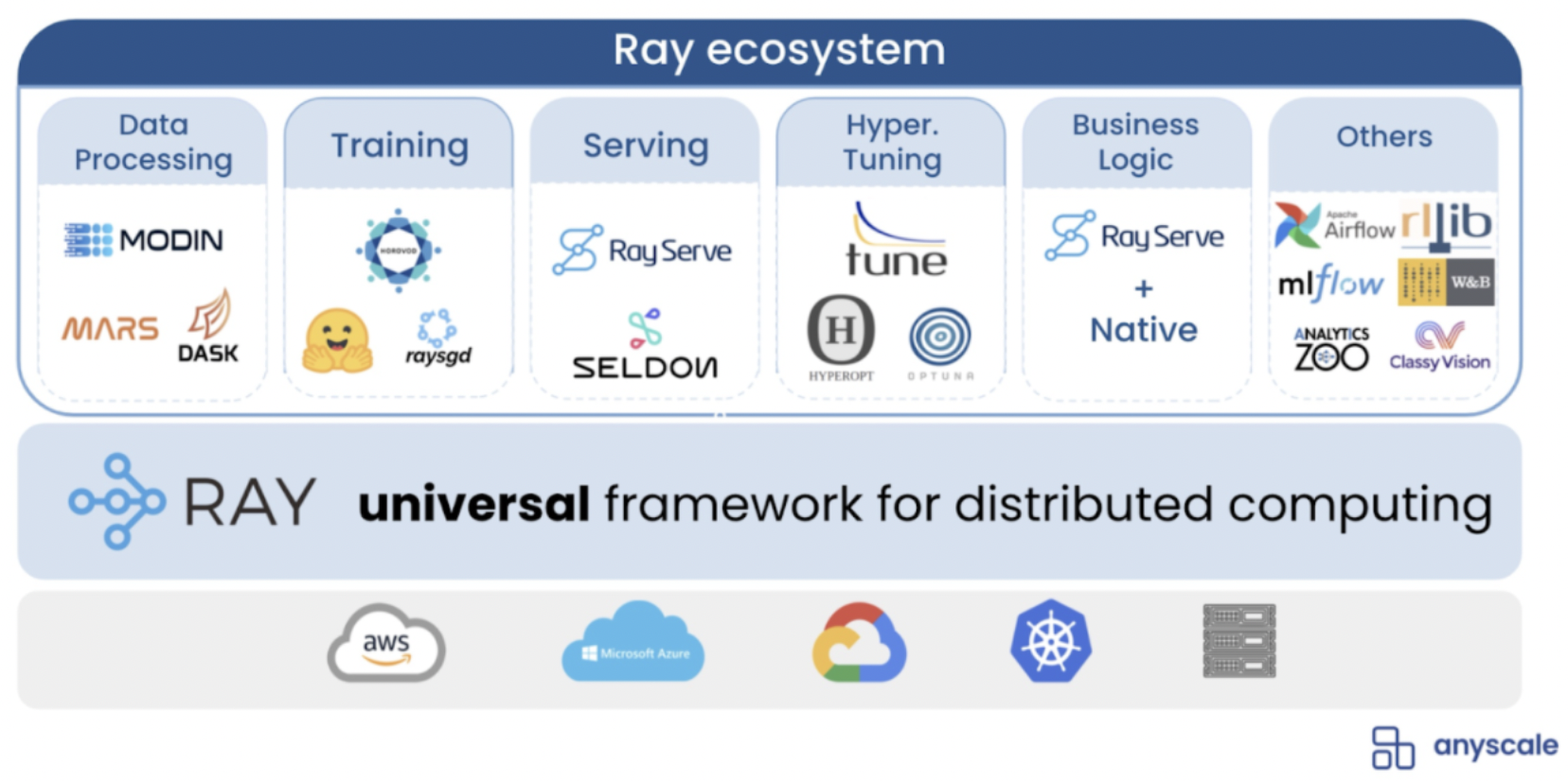Ray Ecosystem, from Ion Stoica’s keynote at Ray Summit 2021.

Ray is an open-source library developed at RISELab from UC Berkeley, which also developed Apache Spark. Ray makes it easy to parallelize and distribute Python code.  The code can then run across any type of cores: a) your own laptop cores, b) cluster in AWS, GCP, or any common cloud.

This rest of the post assumes you already have a PyTorch Lightning model defined, either through vanilla PyTorch Lightning or through PyTorch Forecasting. The parts of code you need to change to make it run on Ray are shown in bold below.

Step 1. Install and import Ray, Ray Plugin for PyTorch Lightning, and Anyscale.  Make sure your PyTorch Lightning version is 1.4.

1
2
3
4
5
6
7
8
9
10
11
12
13
# Install these libraries in your conda environment 
conda install pytorch 
pip install pytorch_lightning==1.4   #required version for ray 
pip install git+https://github.com/jdb78/pytorch-forecasting@maintenance/pip-install  #used at time of writing this blog, check for updates 
pip install ray 
pip install anyscale 
pip install ray_lightning
# Import these libraries in your .py or .ipynb code    
import torch  
import pytorch_lightning as pl   
import pytorch_forecasting as ptf  
import ray 
from ray_lightning import RayPlugin

Step 2. Initialize Ray for the number of cores on your laptop (this is default behavior). Mine had 8 cores.

ray.init()

Step 3. Initialize the Ray Lightning plugin, also for the number of cores on your laptop.

1
2
3
4
5
6
plugin = RayPlugin(
          num_workers=8,  #fixed num CPU
          num_cpus_per_worker=1,
          use_gpu=False,  #True or False
          find_unused_parameters=False, # skip warnings
          )

Step 4. Read sample data which is located in the same github repo as the code. Data is already aggregated into hourly taxi rides per location in NYC.

1
2
3
4
5
6
7
8
# read data into pandas dataframe
filename = "data/clean_taxi_hourly.parquet"
df = pd.read_parquet(filename)

# keep only certain columns
df = df[["time_idx", "pulocationid", "day_hour",
         "trip_quantity", "mean_item_loc_weekday",
         "binned_max_item"]].copy()

Step 5. Convert your data to PyTorch tensors and define PyTorch Forecasting data loaders, like usual. The PyTorch Forecasting data loaders API conveniently folds tensors into train/test backtest windows automatically. Next, in the PyTorch Lightning Trainer, pass in the Ray Plugin. Add plugins=[ray_plugin] parameter below.

1
2
3
4
5
6
7
8
9
10
11
12
13
14
15
16
17
18
19
# convert data to PyTorch tensors and PyTorch Forecasting loaders
# PyTorch Forecasting folds tensors into backtest windows
train_dataset, train_loader, val_loader = \
     convert_pandas_pytorch_timeseriesdata(df)

# define the pytorch lightning trainer
trainer = pl.Trainer(      
      max_epochs=EPOCHS,      
      gpus=NUM_GPU,      
      gradient_clip_val=0.1,        
      limit_train_batches=30,       
      callbacks=[lr_logger, 
                 early_stop_callback],      
      # how often to log, default=50      
      logger=logger,      
      # To go back to regular python - just comment out below      
      # Plugin allows Ray engine to distribute objects     
      plugins=[ray_plugin]
      )

Step 6. Run your code like usual.

1
2
3
4
5
6
7
8
9
10
11
12
13
14
15
16
17
18
19
20
21
22
23
24
25
26
# define a pytorch forecasting model
model = ptf.models.TemporalFusionTransformer.from_dataset(
          train_dataset,   
          learning_rate=LR,      
          hidden_size=HIDDEN_SIZE,      
          attention_head_size=ATTENTION_HEAD_SIZE,      
          dropout=DROPOUT,    
          hidden_continuous_size=HIDDEN_CONTINUOUS_SIZE,
          loss=ptf.metrics.QuantileLoss(),      
          log_interval=10,      
          reduce_on_plateau_patience=4, 
          )

# fit the model on training data
trainer.fit(      
    model,      
    train_dataloaders=train_loader,         
     val_dataloaders=val_loader, 
)

# get best model from the trainer
best_model_path = trainer.checkpoint_callback.best_model_path
best_model = \
ptf.models.TemporalFusionTransformer.load_from_checkpoint(
      best_model_path
)

That’s it! Now your PyTorch Lightning model will run distributed. Behind the scenes, the Ray Lightning Plugin APIs together with Ray are distributing both the data and the models, automatically. The input data is automatically fully sharded, data shards and training functions placed on every distributed node, gradients shared between nodes, one global model produced, and the resulting model is returned as requested type (PyTorch Lightning or PyTorch Forecasting model type).

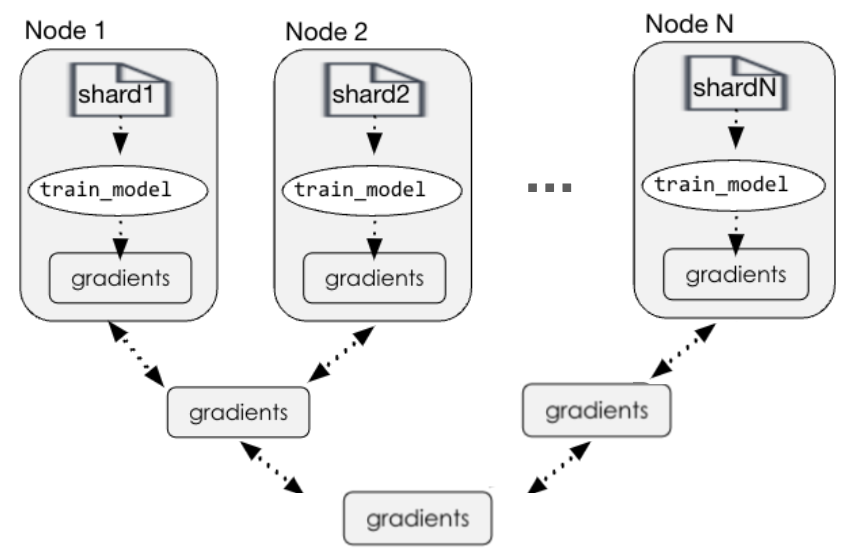What Ray does behind the scenes to distribute learning of global models across N compute nodes. The input data is fully sharded, each node gets the same training functions, gradients are shared between parallel nodes, and one global model is produced. Image by Author.

Previously, I tried to train this model on my laptop, but interrupted the runtime after several hours, since the first epoch still had not finished. After distributing the code with Ray, the same code runs in about 1 hour.

These small tweaks made it possible to train a very accurate DL global forecasting model in about 1 hour on a fairly small compute resource (my laptop). 

Another benefit of Ray is now that the code runs in parallel on my laptop, I can run the SAME code on any cloud using Anyscale, which I’ll show next.

Model training output running on a laptop with 8 cores. iPython %% time output shows it took about 1 hour to train a very accurate forecast.

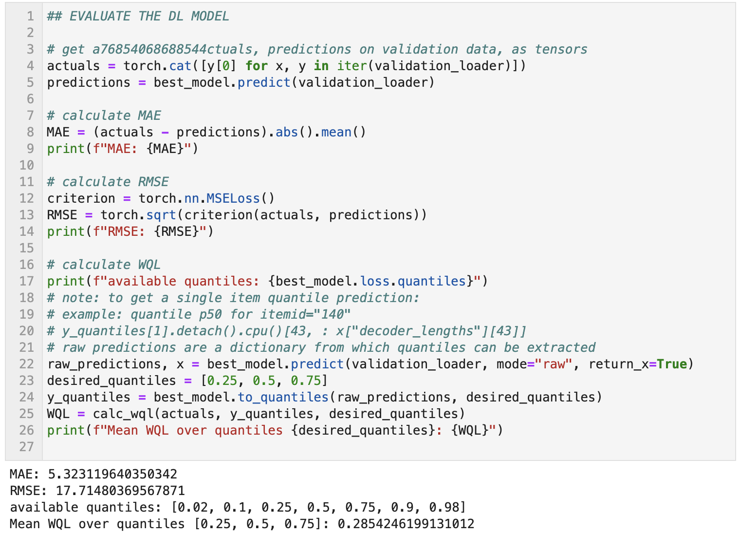Model training output running on a laptop with 8 cores. Accuracy calculated using predictions on hold-out validation data 1 week.

LinkHow to speed up model training and inference in any cloud using Anyscale

Next, to train or do inference faster, you probably want to run that same code on a cloud on bigger instances or across a cluster. In order to use the exact same Ray code on a cloud, (AWS, GCP, …), you need to use either Ray open source cluster or Anyscale which simplifies any cloud setup. 

With Anyscale, you have a choice to either a) do pip installs and github clone on a cluster config, or b) do them at runtime. See cluster or runtime environments for more information. The cluster config is used first, then the runtime config, if specified, will override the cluster config.

The steps to run Ray code on any cloud using Anyscale are:

Step 1. Sign up for Anyscale (see this link) and set up your account (see this link). 

Step 2. Create a cluster configuration. I did this for convenience, since I had a number of atypical, newer ML libraries to install with dependencies. Open your browser to the Anyscale console, and under the Configurations left menu, click the Create new environment button. See picture of Anyscale console below.

1. Cluster environment name.  Give your environment configuration any name.

2. Select a Python version

3. Select a base docker image. I chose

   anyscale/ray-ml:1.9.0-python38-gpu

4. Under Pip packages, see picture below for packages to install and what order.

5. Under Post build commands, see picture below if you would like to install this demo code and data automatically.

6. Click Create button.
   
   Make note of your cluster-config-name:version_number. In the screenshot below, mine is christy-forecast-pytorch:13. You’ll need this for the next step.

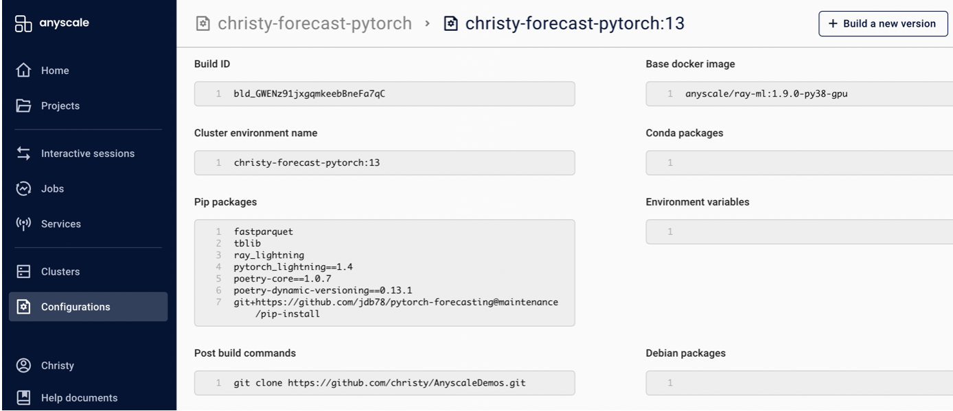Anyscale console, showing Configuration left menu. The main screen shows an example configuration with additional pip installs and github clone on top of the base docker image.

Step 3. Initialize Ray with the name of the cloud cluster and cluster config.

import anyscale

# initialize ray on Anyscale to run on any cloud
# name your cluster on the fly
# set cluster_env parameter = your preconfigured cluster config name
ray.init(
     anyscale://my-cool-cluster, #give your cluster any name
      cluster_env=christy-forecast-pytorch:13,
)

Step 4. Initialize the Ray Lightning plugin with num_workers=N, where N > num cpu on the head node of your cloud cluster. If you specify any number <= N, Anyscale will not scale out. With any number > N, Anyscale autoscaling will trigger automatically, up to limit configured in your account. Set GPU if you have access to a GPU.

plugin = \
       RayPlugin(num_workers=10, 
            num_cpus_per_worker=1, 
            use_gpu=True,
       )

Now, run your python code (or notebook) the way you would normally.  It will automatically run in parallel in any cloud! While your application is running, you can monitor your Cloud Cluster usage in the Anyscale console under Clusters. 

LinkConclusion

This blog demonstrated how easy it is to enable both data and model parallelism for PyTorch Lightning models used for time series forecasting.  Only minimal code changes were required.  Once modified for Ray, the same code can run in parallel on your laptop or in parallel on any cloud through Anyscale.

Full code for the demo is on github.

Thanks to Jan Beitner, author of PyTorch Forecasting, for accepting my Pull Requests and creating a maintenance release, used in this demo.