Reinforcement learning with Deep Q Networks
This series on reinforcement learning was guest-authored by Misha Laskin while he was at UC Berkeley. Misha's focus areas are unsupervised learning and reinforcement learning.
In our last posts we introduced reinforcement learning (RL) intuitively, explained why it’s important, and defined a general mathematical framework for building RL agents. As a recap, we defined the goal of RL algorithms in the following way:
💡 The goal of an RL algorithm is to learn a policy that achieves the maximum expected returns
in its environment.
We know that RL algorithms should maximize expected returns, but what objective should they optimize? For a common machine learning problem like regression, we might optimize the model by minimizing the mean squared error (MSE). A neural network that minimizes the MSE will become better at predicting continuous valued targets given some input data. Can we find a similar notion of “error” that when minimized will result in the agent maximizing rewards?
Yes — and to do so we’ll introduce Q functions. A Q function is just another name for the expected returns and the agent’s goal is to achieve
. Q functions are also known as action-value functions because they predict how much return an agent expects to get if it takes a specific action. Intuitively, a Q function says “if I take action
I think I will get a return of
.”
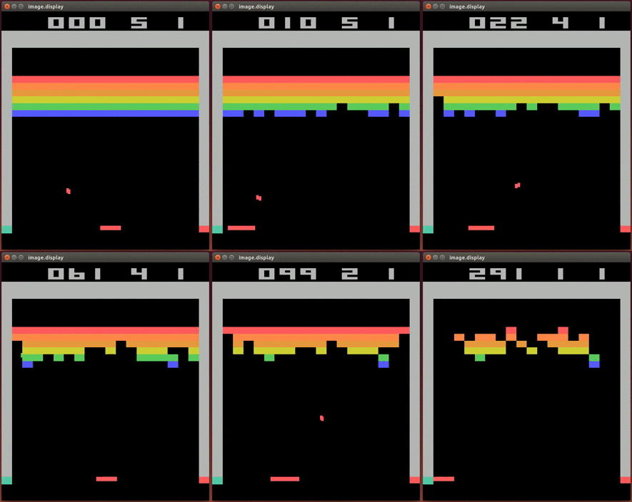
In what follows, we’ll derive the Q learning algorithm and show how it was applied to yield one of the first breakthroughs that started the field of Deep RL: the Deep Q Network (DQN). DQNs were the first AI agents to play video games successfully from images. Below is an example of a DQN agent playing the classic game of Breakout.
 A DQN playing Atari
LinkThe Bellman equation
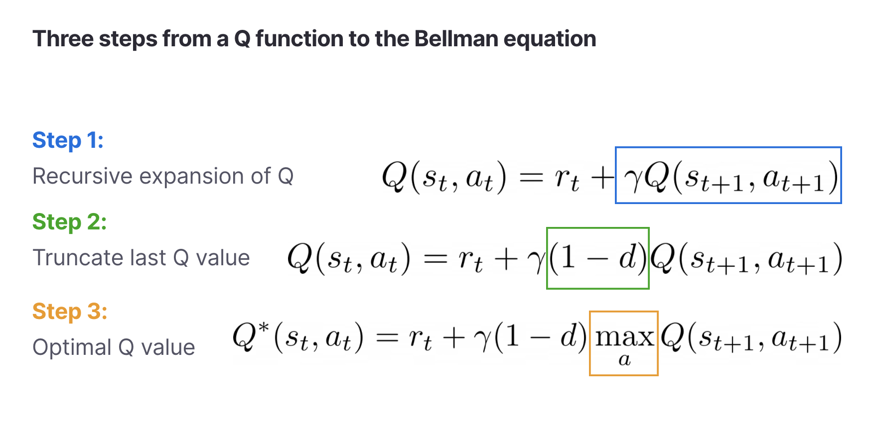
We still don’t know how a Q function translates to a training objective for RL, but we’re not far from the answer. With a few observations we can derive a loss function for RL. Based on the definition where
is a discount factor, we can rewrite a Q function through a following recursive relation. In the below notation
is the done flag, which is false for every step except for the last one of the episode, when the episode ends and done is set to true.

In step (1) we expanded the sum in the definition of Q. In step (2) we need the term because at the final step in the episode the Q function is equal to the last reward, since there are no more rewards in the future. In step (3) we noted that the optimal Q value
is achieved by picking the action that will get the highest returns. This is called the Bellman equation.
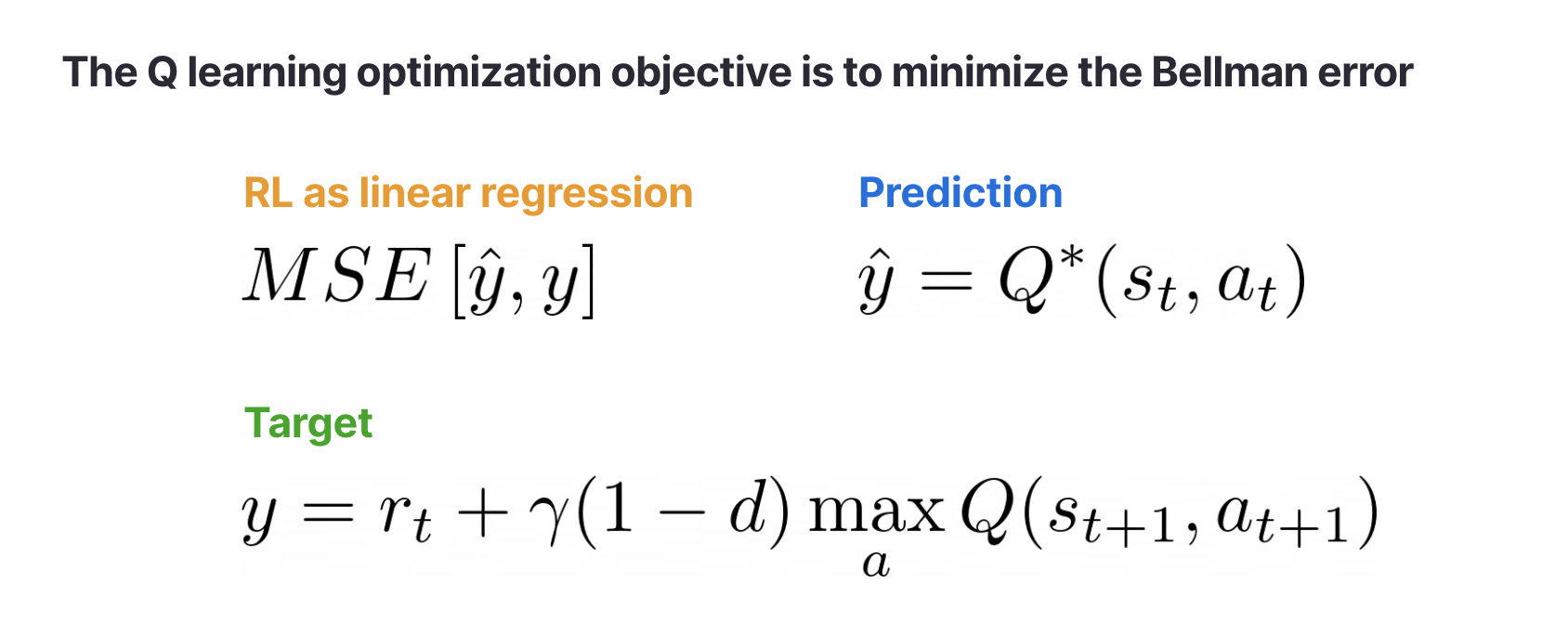
The leap from this equation to an optimization objective is short. If we want to maximize Q, then we need to make sure that the left and right hand sides of the Bellman equation are equal. So to train an RL algorithm we need to minimize a mean squared error, just like in regression problems!

This error is called the Bellman error.
LinkDeep Q Networks (DQNs)
If the state and action spaces are discrete and small, then is just a table with with states as rows and actions as columns. A tabular Q function can be learned by visiting each state with each action and updating the Q values recursively. But suppose we want to control an autonomous vehicle using image input — then the state space becomes huge (the number of possible images) and we can no longer store Q as a table.
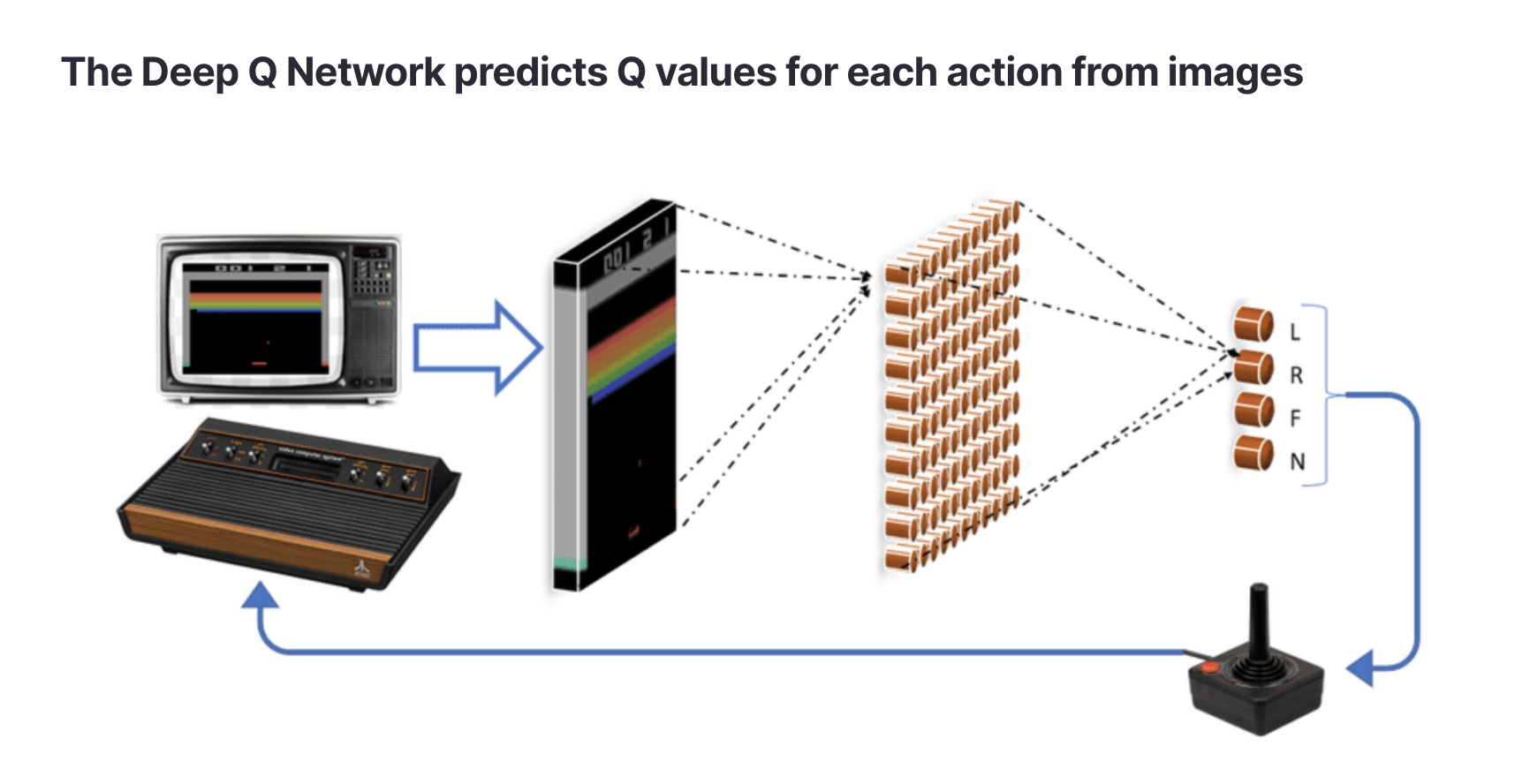
Instead, we’ll approximate Q with a neural network. This is where the “deep” part of Q learning comes in. For simplicity let’s assume that our action space is discrete. Now rather than storing Q as a table, the neural network will input an image (or another type of high dimensional state) and output predictions for the Q values of each action.
 Source: https://arxiv.org/abs/1903.11012
LinkThe Q Network
In torch-like pseudocode a Q network multi-layer perceptron (MLP) might look like this:
1"""
2A network for predicting Q values
3"""
4class Qnet:
5	def __init__(self, action_dim, state_dim, hidden_dim):
6		# simple MLP that outputs Q values for each action
7		self.net = nn.Sequential([nn.Linear(state_dim, hidden_dim), nn.ReLU(),
8															nn.Linear(hidden_dim, hidden_dim), nn.ReLU(),
9															nn.Linear(hidden_dim, action_dim)])
10	def forward(self, x):
11 return self.net(x)LinkComputing the Bellman error
For image input, like Atari, we can use a convolutional neural network instead, but in this example we’ll stick with MLPs for simplicity. The Bellman error can be computed as follows:
1"""
2Computing the Bellman Error given a transition (s, a, r, s_next, d)
3"""
4def BellmanError(network, s, a, r, s_next, d, gamma):
5	# predict Q for all actions from state (s)
6	all_Q = network(s)
7	# extract only Q vals for actions taken (a)
8	Q = all_Q[a]
9	# compute target Q vals for next state (s_next)
10	all_target_Q = network(s_next)
11	# take the highest Q values
12	target_Q = argmax(all_target_Q, dim=1)
13	# Bellman eq right hand side
14	rhs = r + gamma*(1-d)*target_Q
15	# compute Bellman mean squared error
16 return mean((Q - rhs)**2)LinkThe replay buffer
We’ve implemented the Q network and the Bellman error in pseudocode, but where does the transition data (s, a, r, s_next, d) come from? During training we run an agent in an environment and the agent stores all transitions it encounters in a database called the replay buffer. For computing the Bellman error we uniformly sample data from the buffer just like we would in normal supervised learning.
1s, a, r, s_next, d = random_transitions_from_buffer(replay_buffer)LinkEpsilon greedy exploration
Finally, we need to specify how our agent chooses its actions when training. The optimal thing to do would be to pick the action with the highest Q value at each state. However, this would result in limited exploration since the agent would always pick the locally optimal action even if exploring would lead it to higher reward regions in the future (i.e., the exploration problem in RL). To ensure that exploration also happens, we can choose to sometimes take random actions and sometimes take optimal ones. This strategy is known as epsilon greedy.
1def epsilon_greedy_step(state, epsilon, action_dim, network):
2	if uniform(0,1) < epsilon:
3		# random action
4		return randint(action_dim)
5	else:
6		# greedy action
7 return argmax(network(state))LinkConclusion
We’ve described Q learning and DQNs. A scaled up variant of this simple algorithm was used to achieve the breakthrough Atari results in 2013 that catalyzed the field of Deep RL. Other algorithms that are now making their way into practical applications like SlateQ for recommender systems are descendants of the simple idea of Q learning by minimizing the Bellman error.
In the next entry in this series on RL, we'll cover some practical tips for training Deep Q Networks. Or, explore these other RL resources:
Register for the upcoming Production RL Summit, a free virtual event that brings together ML engineers, data scientists, and researchers pioneering the use of RL to solve real-world business problems
Learn more about RLlib: industry-grade reinforcement learning
Check out our introduction to reinforcement learning with OpenAI Gym, RLlib, and Google Colab
Get an overview of some of the best reinforcement learning talks presented at Ray Summit 2021