The reinforcement learning framework
This series on reinforcement learning was guest-authored by Misha Laskin while he was at UC Berkeley. Misha's focus areas are unsupervised learning and reinforcement learning.
In the previous blog post in this series, we provided an informal introduction to reinforcement learning (RL) where we explained how RL works intuitively and how it’s used in real-world applications. In this post, we will describe how the RL mathematical framework actually works and derive it from first principles.
LinkThe components of an RL algorithm
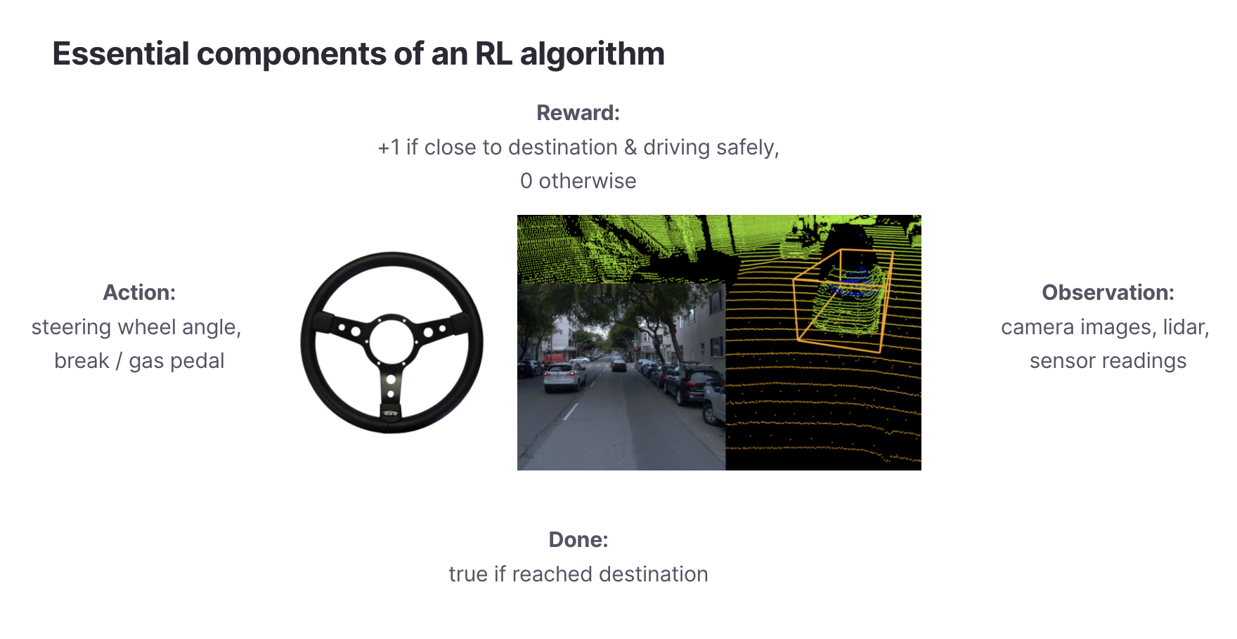
 The essential components of an RL algorithm. Source for AV image: https://github.com/waymo-research/waymo-open-dataset
First, we need to start with defining the problem setting. RL algorithms require us to define the following properties:
An observation space
. Observations are the data an RL agent uses to make sense of the world. An autonomous vehicle (AV) may observe the world through cameras and Lidar.
An action space
. The action space defines what actions an RL agent can take. An AV’s action space could be the steering wheel angle as well as the gas and break pedals.
A reward function
. The reward function labels each timestep with how favorable it is for the overall metric that we want to optimize. For AVs, the reward function could be whether the car is closer to its destination and is driving safely.
A terminal condition
. This is the condition that determines the length of single episode of an RL loop. It is either a fixed time amount (e.g., 1000 steps) or is triggered when a success condition is met (e.g., AV car arrived safely or user purchased a recommended item).
LinkThe goal of an RL algorithm

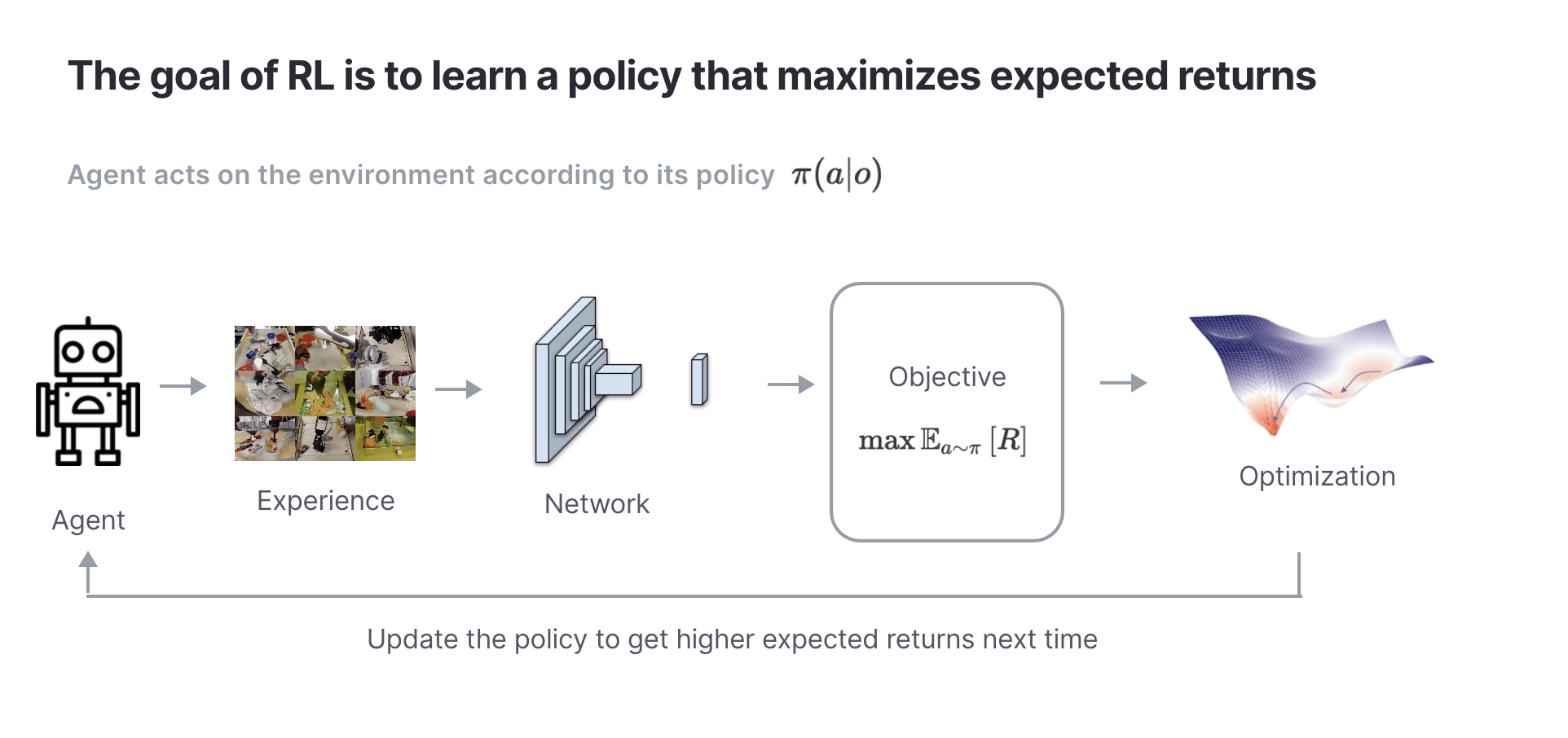
Now that we understand the problem setting, we need to define what an RL algorithm is optimizing. The goal of RL algorithms is quite simple: learn a policy that maximizes the total rewards (also known as return)
within an episode. Intuitively, the policy is the RL agent. It outputs an action given the agent’s current observation.
Unfortunately there is a chicken-and-egg problem with the current goal. In order to achieve the RL agent needs to see the future returns, but to see future returns the policy needs to act on the environment by which point the returns are no longer in the future. How can the agent choose an action in a way that achieves
before actually acting in the environment?
This is where the very important concept of expectation comes in. The RL agent doesn’t maximize the actual rewards. Instead it forms an estimate of what it thinks will be in the future if it acts according to
. In other words, the goal of the agent is to achieve
, not
. This concept of expectation is at the core of all RL algorithms. In the next post, we will show how this objective leads to Q-learning, but in the meantime we can state the main goal of RL as:
💡 The goal of an RL algorithm is to learn a policy
that achieves the maximum expected returns
in its environment.
LinkThe RL loop

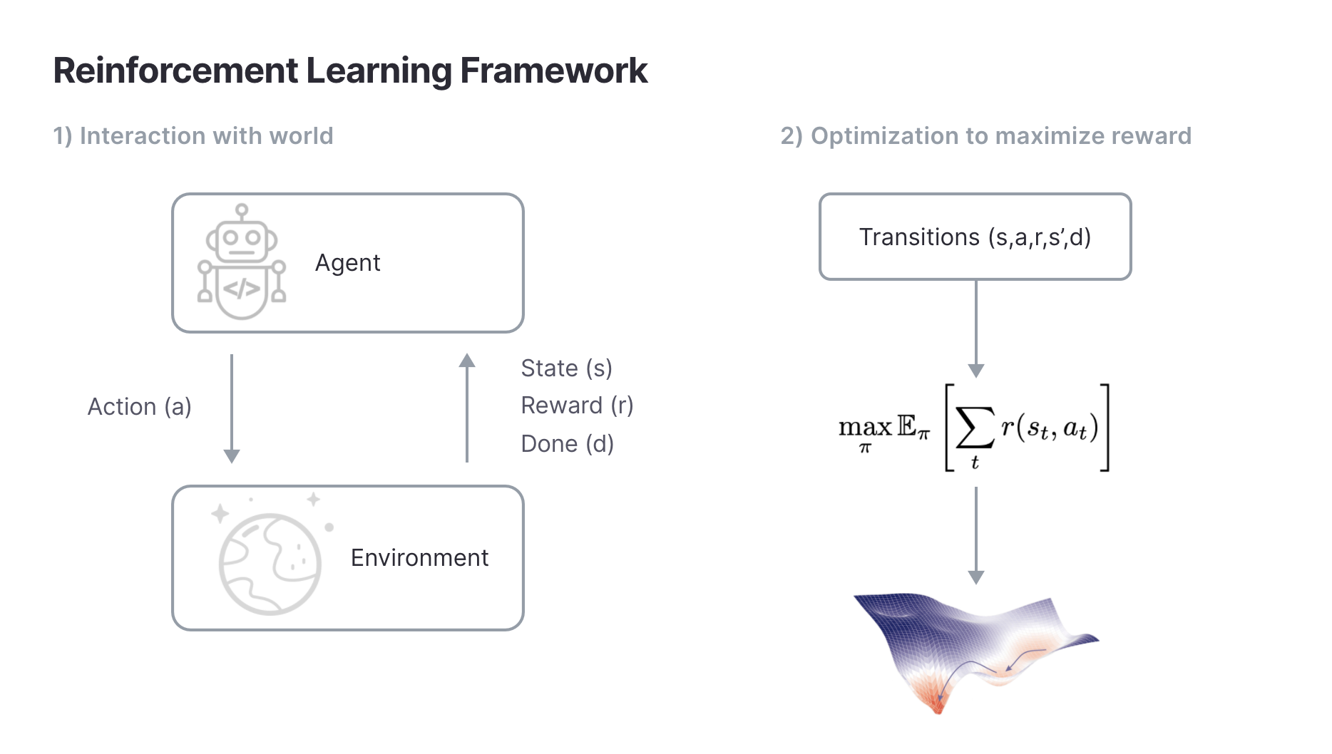
Having specified the components and goal of an RL algorithm we can define the RL loop. At each timestep, the agent observes its world, acts on it, and receives a reward. This process repeats until the terminal condition has been reached. Separately, the agent updates its policy using the data it has collected so far to learn a policy
that maximizes rewards.
A small but important detail worth noting is that when considering the return most RL algorithms introduce an additional parameter called the discount factor. The discount factor helps RL algorithms converge faster by prioritizing near-term rewards so that the return is weighted by the discount
. Usually
is set to be close to one (e.g.,
) to prevent short-sightedness in the RL algorithm.
The intuitive interpretation of the discount factor is that it sets the length of the time horizon that an RL agent will consider when maximizing rewards. For example, a discount factor of will make the agent maximize returns over approximately 100 steps (since
will be close to zero). In other words, the discount factor is a hyperparameter that determines the agent’s reward horizon. Values of
closer to zero are easier to optimize since the agent will only care about near-term returns, while values that are closer to one will make the agent maximize returns over long time horizons but are harder to optimize. Most practical RL algorithms include a discount factor.
💡 The goal of most practical RL algorithms is to maximize expected discounted returns
.
LinkConclusion
We have shown the mathematical framework for designing RL algorithms. The thing to note about this framework is that it is very general. As long as you can define an observation space, action space, and a reward function, you can build an RL algorithm and optimize it to learn a policy that maximizes expected returns. In general, RL doesn’t make any assumptions about the underlying problem it’s trying to solve, which is why it is so broadly applicable across AV navigation, recommender systems, resource allocation, and many other useful problems.
Stay tuned for the next entries in this series on RL, where we'll explore RL with Deep Q Networks. In the meantime, there's plenty more to explore in the RL universe:
Register for the upcoming Production RL Summit, a free virtual event that brings together ML engineers, data scientists, and researchers pioneering the use of RL to solve real-world business problems
Learn more about RLlib: industry-grade reinforcement learning
Check out our introduction to reinforcement learning with OpenAI Gym, RLlib, and Google Colab
Get an overview of some of the best reinforcement learning talks presented at Ray Summit 2021


