Cut coding agent costs by 90%: Secure LLM serving with Ray + vLLM on Anyscale

Coding agents repeatedly send repository context, instructions, tool results, and conversation history to generate actions. That work is also some of the most sensitive you do: your source, your internal docs, your architecture decisions, leaving your perimeter on every keystroke. Owning the runtime is how that stays yours: the code, the traces, and the usage data that eventually could help you post-train those models to make them more tailored to your team.

Beyond data privacy, paying for closed-source LLMs by the token also means a linearly growing bill per developer, per request, with no way to derive efficiencies of scale as the team and number of agents grows. Owning the runtime also shifts that by enabling a team to share the underlying GPUs. BMW found the cost-benefit of moving from API to in-house inference with as few as 8 developers. But building and managing your in-house LLM serving platform for coding comes with its own operational challenges when running GPU clusters. 

As far as costs, key findings from our cost model show that self-hosting costs a fraction of per-token API pricing per developer:

• Always-on serving: About $2,920 per month, or about $58 per registered developer.

• Work-hours-only serving: About $840 per month, or about $17 per registered developer.

• API baseline: An active developer routinely runs up about $800 per month in equivalent Claude Code API costs.

These figures assume roughly $4 per GPU-node hour for an RTX PRO 6000 and 50 registered developers sharing one GPU. They are planning projections rather than a TCO; the full assumptions and caveats are in the cost comparison section below.

In addition to cost savings, optimizing the serving infrastructure yields measurable performance gains.

Key findings from our empirical evaluations demonstrate significant performance improvements:

• 8.0x faster compilation with compile-cache restoration. In a no-MTP NVFP4 setup, compilation time dropped from 48.5 to 6.0 seconds.

• 3.79x higher request throughput with CPU KV-cache tiering. Adding a 512 GiB CPU tier in a single-replica GLM-5.2 evaluation increased the cached share of prompt tokens from 6.1% to 74.9% across 58 common prompts, reducing median time-to-first-token (TTFT) from 48.4 to 9.2 seconds.

• 1.86x higher output throughput with speculative decoding. Multi-token prediction (MTP) increased output throughput from 65 to 121 tokens/s. 

• 2.87x faster output generation with CUDA graphs enabled. Client-observed token throughput increased from 15.9 to 45.6 tokens/s compared with running in eager mode.

This guide provides a step-by-step roadmap covering model and hardware selection, service deployment, single-replica tuning, autoscaling with cache-aware routing, and multi-model operations.

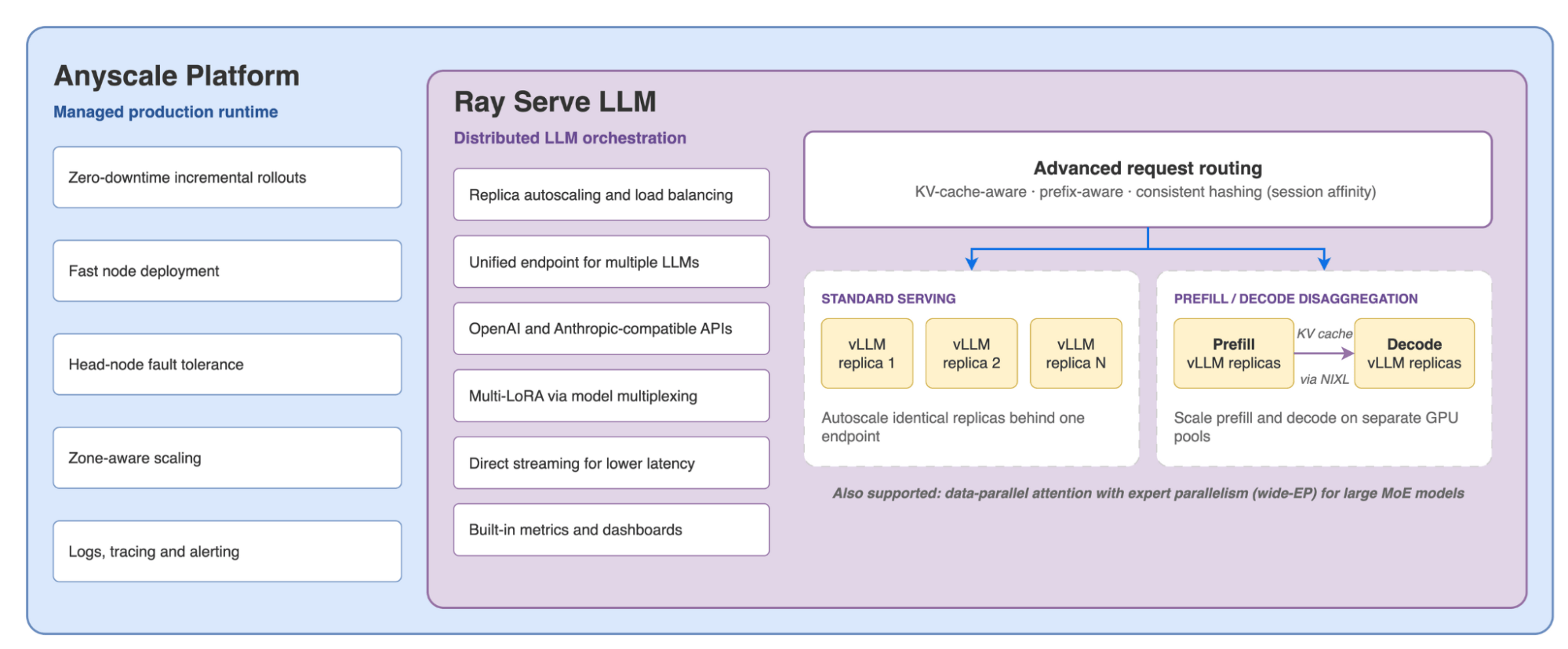Figure 1. The LLM serving stack on Anyscale: vLLM runs the model, Ray Serve LLM orchestrates and routes across replicas, and Anyscale manages the production runtime.

How the LLM serving stack operates:

• vLLM: the inference engine that loads the model on GPUs and generates tokens.

• Ray Serve LLM: the orchestration layer that scales, routes and load-balances requests across many vLLM replicas behind one OpenAI- and Anthropic-compatible endpoint, including advanced patterns like prefill/decode disaggregation.

• Anyscale Platform: the managed production runtime that provisions GPUs, autoscales nodes (including scale-to-zero), and adds reliability and observability such as zero-downtime rollouts, fault tolerance, logs, tracing and alerting.

To make this path reproducible, we created the LLM serving for coding agents code repository.

The repository is organized into five runnable parts:

• Part 1: Deploy: Launch and validate a baseline Anyscale service.

• Part 2: Connect: Connect Claude Code, Codex, and Cursor through their native APIs.

• Part 3: Optimize: Tune GPU usage, caching, decoding, and autoscaling.

• Part 4: Route: Route between the open model and Claude with LiteLLM.

• Part 5: Roll out: Configure zero-touch deployment for a team.

LinkHow coding agents shift the serving workload

LinkCoding agents produce far more than chat traffic

Coding-agent prompts combine system instructions, repository context, tool definitions, diagnostics, and conversation history—often to produce only a short tool call or edit. This makes the workload prefill-heavy, with large inputs dominating time to first token (TTFT).

Most of that context is repeated across turns, creating strong opportunities for automatic prefix KV-cache reuse. At team scale, correlated bursts add another challenge. A high-performance platform must therefore balance four goals: low TTFT, smooth token streaming, high cache reuse, and elastic capacity.

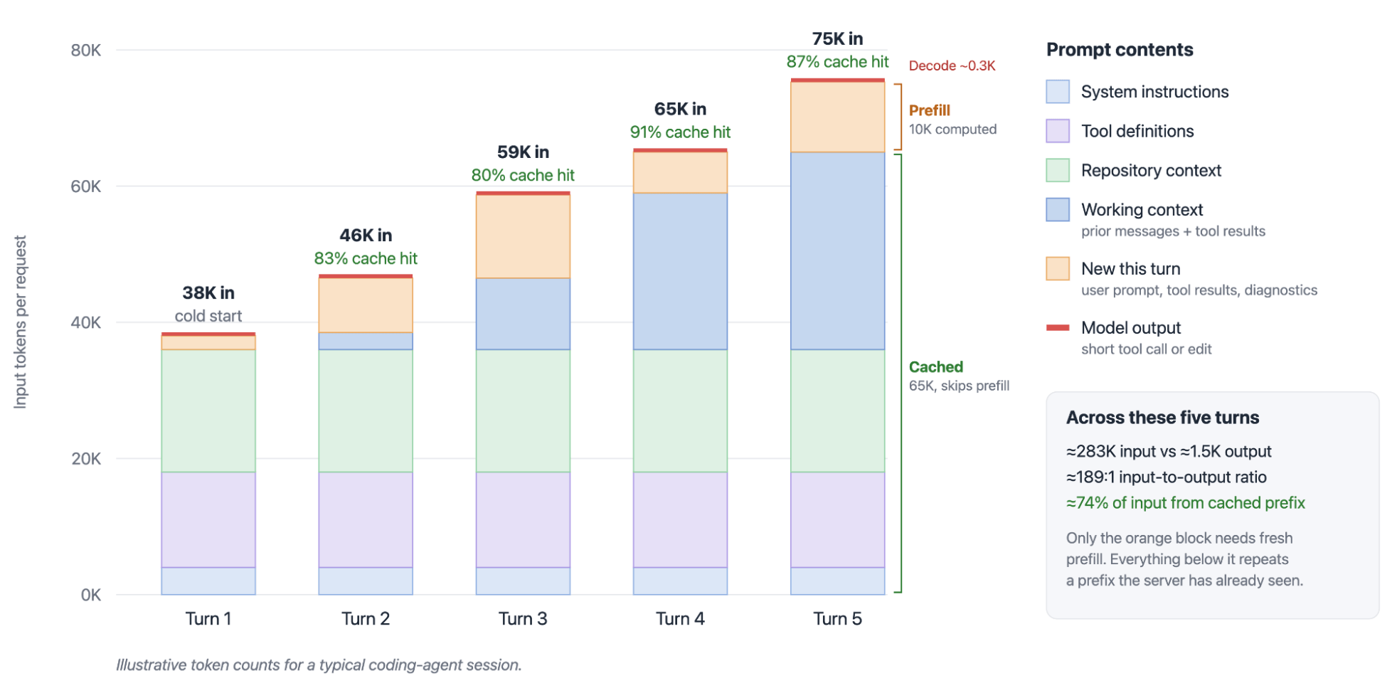Figure 2. Illustrative coding-agent session: each turn re-sends a large, mostly repeated prompt to produce a short output. Only the new content each turn (orange) needs fresh prefill; the rest can be served from the KV cache.

Coding-agent harnesses act as API clients. When configured with custom endpoints, the local harness—or, for hosted clients such as Cursor, its cloud backend—sends requests to a compatible model server instead of relying on the default hosted model. Because these clients use different API schemas and endpoints, the serving infrastructure must expose the corresponding routes. The repository's client integration guide configures these three paths:

Hosting an open-weight model on Anyscale can provide several benefits:

• Reduce cost: Lower marginal token cost when utilization is high enough to offset fixed infrastructure expense.

• Control capacity: Reduce dependence on a single provider's rate limits while managing your own capacity and queues.

• Security and data control: Keep more of the inference path inside your network.

• Reduce model-provider lock-in: Gain control over model and serving upgrades.

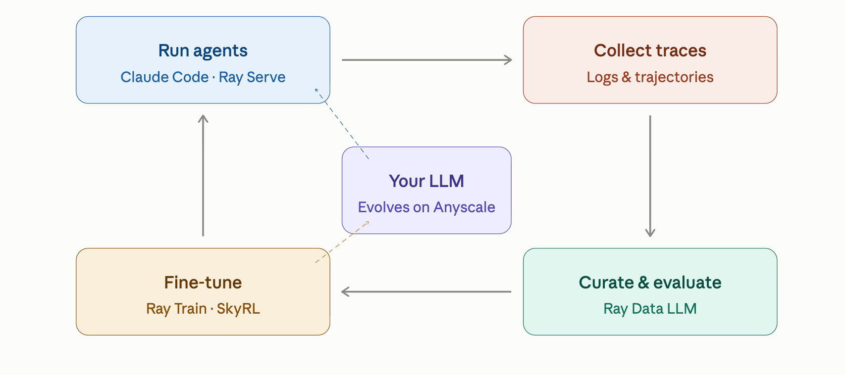
• Evolve the LLM with your own data: Create a data flywheel by capturing approved agent traces, curating and evaluating them with Ray Data, and post-training with Ray Train or an RL framework.

Community and transparency: Leverage the open ecosystem to understand and customize model behavior.

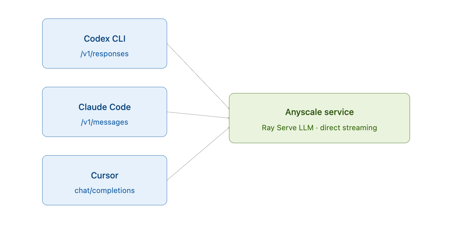Figure 3. Direct streaming enables the Ray Serve LLM to connect with coding agents across various endpoints.

LinkRay Serve LLM scales it for production

While vLLM handles core inference optimizations—such as prefix caching, chunked prefill, quantization, speculative decoding, and model parallelism—a robust deployment needs more. Ray Serve LLM adds a production layer to:

• Scale replicas across multi-GPU environments.

• Route requests intelligently based on load and cache state.

• Expose OpenAI- and Anthropic-compatible APIs.

• Stream tokens from replicas through HAProxy while bypassing the legacy Python ingress hop.

• Centralize metrics for services, models, and GPUs.

• Ergonomic builders for complex, multi-node deployments like Wide-EP and prefill disaggregation

A published recent Ray Serve LLM benchmark measured cumulative throughput gains of up to 4.4x on prefill-heavy workloads and 24.8x on decode-heavy ones relative to an older, unbatched Ray Serve LLM baseline after introducing HAProxy, direct streaming, and RayExecutorV2. On Anyscale, Ray Serve LLM adds managed autoscaling, observability, and fault tolerance around the inference engine.

LinkDeploy an LLM for coding agents

A practical deployment has four steps:

1. Select a model based on task quality and serving footprint.

2. Select hardware and a parallelism strategy.

3. Configure the vLLM engine and Ray Serve deployment.

4. Deploy the service and validate each coding client.

LinkStep 1: Select an LLM for task success, not leaderboard rank alone

Open-weight model quality is moving quickly. Agent leaderboards such as the Agent Arena ranking for open-source models are fine places to start, and model families including Qwen, DeepSeek, Kimi, and GLM increasingly target coding and tool use. However, public rankings are only a starting point, and Anyscale LLM experts can help you select the best model for your specific workloads.

Common benchmarks include SWE-bench for resolving real repository issues, Terminal-Bench for terminal tasks, Toolathlon for long-horizon multi-tool workflows, τ-bench for conversational tool use, CyberGym for vulnerability analysis, and GDPval-AA v2 for professional knowledge work. Scores often reflect the full agent system—not only the model—so compare results only when benchmark versions and evaluation setups match.

Evaluate candidate models on your own work:

• Multi-file edits and repository navigation.

• Structured tool calls over several turns.

• Long-context instruction following.

• Debugging and test repair.

• Latency and number of turns required to finish a task.

A smaller model that completes common work in one reliable turn can be cheaper than a larger model that needs more GPUs. A stronger model may be cheaper for difficult tasks if it avoids retries. Measure cost per successful task, not only cost per million tokens.

LinkStep 2: Fit weights, runtime memory, and KV cache to the hardware

GPU memory holds model weights, the KV cache, temporary activations, CUDA graphs, and runtime overhead. Weight memory is mostly fixed and scales with parameter count and precision, so weight quantization can be essential when unquantized weights constrain the deployment. The KV cache stores attention state for active requests and grows with context length and concurrency. For long-context coding-agent workloads, KV cache quantization can likewise reduce per-token memory. Quantizing both, when supported and quality-validated, leaves more room for concurrent long requests.

When selecting a quantization strategy, consider the following formats:

• FP8: A strong option for both weights and the KV cache when supported by the hardware and runtime. It roughly halves raw storage compared with BF16; quality remains model-, task-, and calibration-dependent.

• NVFP4: On NVIDIA Blackwell GPUs, this format halves raw storage for quantized tensors compared with FP8. Whole-checkpoint savings are smaller because some modules and metadata remain at higher precision; the tested Qwen checkpoint used approximately 22 GB versus 27 GB for FP8, a reduction of about 19%.

• MxFP4: An open alternative for 4-bit precision, used by models such as gpt-oss.

Note: Runtime setup and GPU architecture dictate the extent of hardware acceleration. While NVIDIA's Qwen3.6-27B-NVFP4 weights are deployed here, the pinned vLLM release relies on a Marlin fallback instead of a native kernel for dense NVFP4 on RTX PRO 6000 hardware. Furthermore, because NVFP4 KV caching is not supported on this device, the system defaults to an FP8 KV cache.

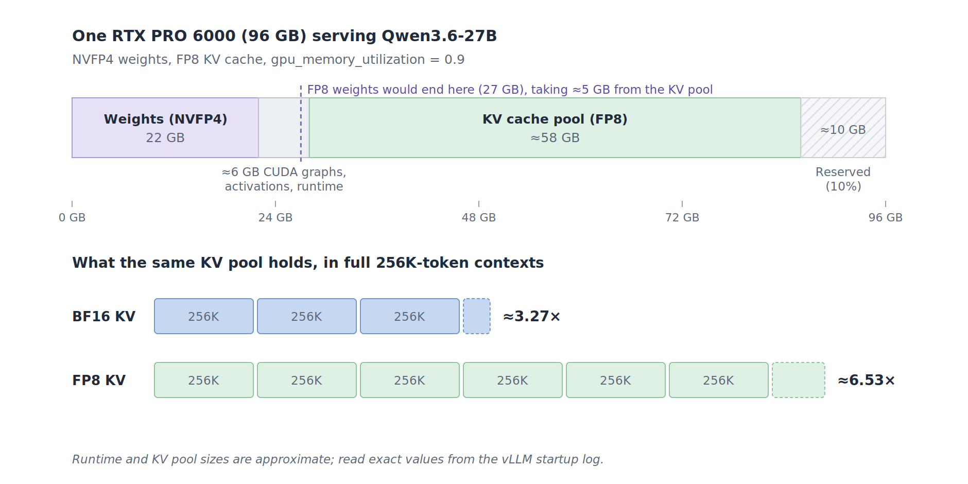Figure 4. Illustrative GPU memory layout: NVFP4 weights leave most memory for KV cache, and FP8 KV fits about twice as many full contexts as BF16.

LinkStep 3: Configure the engine for the model and workload

A correct serving configuration is model-specific. In addition to memory and parallelism, it must use the right chat template, reasoning parser, tool-call parser, multimodal limits, and context length.

The repository's Qwen serving implementation configures one GPU per replica, a 256K context limit, FP8 KV cache, local prefix caching, chunked prefill, and Qwen-specific reasoning and tool parsers. The following excerpt shows the relevant engine arguments; the implementation configures speculative decoding and compile-cache behavior separately:

engine_kwargs = {
    "tensor_parallel_size": 1,
    "max_model_len": 262144,
    "gpu_memory_utilization": 0.9,
    "max_num_seqs": 32,
    "max_num_batched_tokens": 8192,
    "enable_prefix_caching": True,
    "kv_cache_dtype": "fp8",
    "quantization": "modelopt",
    "reasoning_parser": "qwen3",
    "tool_call_parser": "qwen3_coder",
    "enable_auto_tool_choice": True,
    "limit_mm_per_prompt": {"image": 4, "video": 0},
}

max_model_len caps a single request's context. max_num_batched_tokens serves as a scheduler budget for chunked prefill. Meanwhile, max_num_seqs restricts engine concurrency. 

LinkStep 4: Enable direct streaming and connect the clients

The repository's always-on service configuration enables HAProxy and direct streaming at the service level:

env_vars:
  RAY_SERVE_ENABLE_HA_PROXY: "1"
  RAY_SERVE_LLM_ENABLE_DIRECT_STREAMING: "1"

Follow the repository's coding-agent connection tutorial. First, deploy the optimized always-on service:

anyscale service deploy -f service-always-on.yaml --working-dir .

Then copy its public base_url and bearer token from Anyscale Console → Services → Query. The agent executes tools locally, but model requests—including instructions, repository context, conversation history, and tool results—and streamed model responses pass through the service.

Claude Code

Export the service URL and token, then run the repository's claude-service.sh:

export ANYSCALE_BASE_URL=<base_url>/v1
export ANYSCALE_API_KEY=<token>
./claude-service.sh

The launcher passes the service root to Claude Code as ANTHROPIC_BASE_URL and supplies the token through ANTHROPIC_AUTH_TOKEN.

Codex

From the same directory, run codex-service.sh:

./codex-service.sh

It registers the /v1 URL as a custom provider, selects wire_api="responses", and sends the bearer token to /v1/responses.

Cursor

Follow the tutorial's Cursor setup and enter these values under Cursor Settings → Models → OpenAI API Key:

Override OpenAI Base URL:  <base_url>/v1
OpenAI API Key:            <token>
Custom model:              qwen3.6-27b

LinkOptimize one replica for coding-agent traffic

LinkBenchmarking latency against defined SLOs

For comprehensive definitions of TTFT, ITL, TPOT, prefill, decode, and goodput, refer to Anyscale's LLM metrics guide.

Rather than focusing solely on raw token throughput, prioritize goodput, the proportion of requests meeting target latency SLOs. While aggressive batching elevates overall throughput, it can negatively impact interactive streaming performance.

LinkReplay real agent sessions for benchmarks

Uniform synthetic prompts fail to capture a true agent loop. Real-world traffic combines long and short turns, repeated prefixes, tool-execution waits, and heavy-tailed session lifetimes. To accurately test your setup, convert your Claude Code JSONL sessions into timestamped request streams that preserve prompt growth and inter-turn delays. If you aren't collecting your own sessions yet, you can use the public WekaTrace Claude Code agent-session corpus.

For each candidate configuration, collect:

• TTFT, TPOT, ITL, and end-to-end latency distributions.

• Completed agent turns and successful tasks.

• Input/output tokens and cached-prompt-token fraction.

• Queue depth, preemption, KV eviction, and GPU utilization.

• Tool-call errors and malformed responses.

LinkApply optimizations in dependency order

The single-GPU measurements below use one RTX PRO 6000. Most decode results were recorded using real Claude session prompts averaging about 73K tokens. Each row isolates a different knob; the gains are not cumulative.

1. Quantize weights to fit the model efficiently. Weight quantization can turn a multi-GPU deployment into a one-GPU deployment, removing inter-GPU communication and freeing memory for KV cache. The benefit depends on the GPU's native kernels and the checkpoint's calibration. Treat every precision change as both a performance and quality change.

2. Quantize the KV cache when supported. The optimized deployment uses FP8 KV cache. Capacity calculations estimated KV storage equivalent to approximately 3.27x 256K-token contexts with BF16 KV and 6.53x with FP8 KV on the tested 96 GB GPU. 

3. Keep CUDA graphs enabled for production. Eager mode launches operations with more CPU involvement and is useful for debugging. CUDA graphs capture repeatable GPU work and reduce launch overhead. Disabling eager mode (keeping CUDA graphs enabled) increased the output rate from 15.9 to 45.6 tokens/s.

4. Test speculative decoding against target workloads. Multi-token prediction proposes and verifies several future tokens simultaneously to reduce TPOT; the num_speculative_tokens parameter controls the number of draft tokens predicted (for example, setting it to 3 to predict three tokens ahead). However, net speedup depends on acceptance rates and verification overhead. At concurrency 8, predicting three tokens yielded 99 output tokens/s and 0.50 turns/s—outperforming two tokens (80 tokens/s, 0.50 turns/s)—whereas predicting four tokens degraded performance to 74 tokens/s. Higher speculative depth is not inherently better. Prioritize output accuracy: upstream issues note corrupted tool calls when combining MTP with prefix caching. Verify client, model, parser, and vLLM compatibility with multi-turn regression tests before enabling MTP.

5. Streamline initialization to separate cold starts from steady-state serving. Model download, weight loading, engine compilation, and replica readiness are distinct phases that impact deployment speed. Compile caches are sensitive to the exact software version, GPU architecture, model, parallelism, and flags, meaning a stale cache can fail or silently degrade performance. While RunAI Streamer reduced earlier weight-load times, the repository's incompatibility matrix documents a known conflict between its loader path and MTP in the tested vLLM version.

In practice, first establish correct tool use with speculative decoding disabled; use eager mode only as needed for debugging. Once correctness is verified, enable the intended quantization and context length, followed by CUDA graphs. From there, tune chunked prefill and test speculative decoding. Finally, optimize the cold start and rerun the full correctness and load suite.

LinkModel cost comparisons

The repository's cost model and assumptions assume roughly $4 per GPU-node hour for the RTX PRO 6000 shape, with 50 registered developers sharing a single GPU. Based on these assumptions:

Claude pricing via Azure Marketplace on Microsoft Foundry follows Claude Opus 5 rates: $5.00 per million tokens (MTok) for standard input, $0.50/MTok for cache reads, and $25.00/MTok for output.

An active developer routinely runs up $800 per month in equivalent Claude Code API costs. This aligns with industry benchmarks, including Pylon's observations of power users reaching $800/month and another similar estimate of $1,199.79 over 30 days. Public trace telemetry confirms that coding agent workloads are heavily skewed toward input tokens:

• The WekaTrace dataset indicates a 117:1 input-to-output token ratio.

• SyFI TraceLab's Claude trace documents a 269:1 ratio with a 95.2% prompt cache hit rate.

Factoring in SyFI's 95.2% cached input rate (billed as cache reads) and treating the remaining 4.8% as five-minute cache writes, Opus 5 pricing translates an $800 monthly spend into approximately 922M input tokens and 3.43M output tokens per developer. For an engineering team of 50 developers, overall API usage totals roughly $40,000 and 171M output tokens per month.

The $40,000 monthly figure serves purely as an API expenditure benchmark rather than a direct indicator of potential infrastructure savings. Because brief, configuration-specific decode tests ignore prefill overhead, request queuing, overall GPU utilization, latency-SLO targets, and variations in model quality, they cannot reliably forecast real-world worker capacity.

Similarly, per-developer GPU cost calculations represent preliminary planning projections instead of a total cost of ownership (TCO) or service-level commitment. To accurately determine required replica counts and net savings, evaluate sustained trace-replay goodput against target latency SLOs and task success rates, then factor in additional platform operational overhead.

LinkScale with autoscaling and cache-aware load balancing

LinkSeparate engine limits, admission limits, and autoscaling targets

The repository's autoscaling configuration provides one concrete starting point, while Anyscale's parameter-tuning guide explains how to tune it. Three controls serve different purposes:

• The vLLM max_num_seqs setting bounds sequences admitted by an engine.

• Ray Serve's max_ongoing_requests bounds work sent to a replica.

• The target_ongoing_requests setting tells the autoscaler when to add replicas.

Here is the step-by-step process for setting up auto-scaling for LLM deployments serving coding agents:

1. Identify peak KV-cache capacity: Check server startup logs to determine the maximum concurrent sequences supported at your maximum context length (e.g., 256K context windows typically sustain around 20 concurrent streams).

2. Estimate practical workload concurrency: Adjust the sequence limit based on your average prompt size. For instance, with an average prompt length of 85K tokens, scale the target using (256K / 85K) x 20 to establish a target of roughly 60 concurrent requests.

3. Set hard admission bounds: Match the engine's scheduler capacity (max_num_seqs in vLLM) and the deployment guard (max_ongoing_requests in Ray Serve) to this calculated upper limit (e.g., 60).

4. Establish autoscaling triggers: Configure target_ongoing_requests roughly 20–30% lower than the admission ceiling (e.g., 40) to initiate replica scaling before requests queue up.

5. Track metrics and refine parameters: Continuously evaluate system goodput and queuing. Reduce concurrency thresholds if prompt lengths approach the 256K ceiling to preserve tail latency as memory headroom narrows.

For coding agents, we recommend using Ray Serve LLM's KVAwareRouter or consistent hashing (session affinity). KV-aware routing combines prefix cache reuse with token-load-aware routing. However, note that KV-aware routing is currently only compatible with Codex. For other clients or incompatible setups, fall back to consistent hashing to maintain session stickiness.

As detailed in the blog, the router uses KV cache overlap to estimate how much prefill can be skipped, then estimates the work the engine still has to do:

remaining prefill = incoming input tokens - reusable cached tokens
token-load score = weighted remaining prefill + active prefill + ongoing decode

The router selects the replica with the lowest weighted score and may trade some cache reuse for more balanced token load. On heterogeneous coding-agent traces, this can improve TTFT, TPOT, and throughput relative to maximizing cache reuse alone.

LinkExtend useful cache lifetime with KV cache offloading

When a developer pauses to review code or write a prompt, other team traffic may evict their session's blocks from limited GPU memory. KV-cache offloading moves inactive blocks to larger CPU-memory or local-storage tiers so they can be restored instead of fully recomputed. For coding agents, offloading preserves session context when a user steps away and returns hours later—the history is retrieved from CPU/disk instead of recomputed, so they resume with a fast TTFT. 

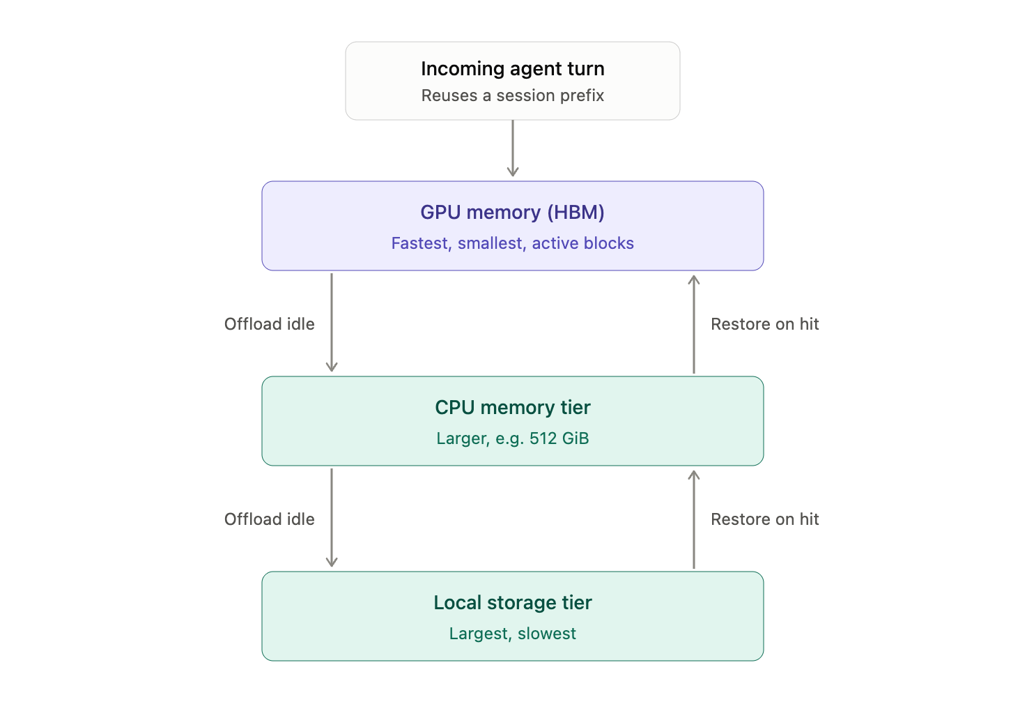Figure 5. KV cache offloading: idle blocks move to CPU or disk and are restored on reuse instead of being recomputed.

In an internal benchmark on a GLM-5.2 workload, adding a 512 GiB CPU KV-cache tier alongside GPU prefix caching significantly improved throughput and latency over GPU caching alone. Evaluated using a single node equipped with 8xRTX PRO 6000 GPUs (tensor parallelism of eight, NVFP4 weights, and FP8 KV cache), the benchmark replayed a seeded workload over a nominal 900-second window.

Key operational takeaways include:

• Throughput Improvement: Overall request throughput increased by 3.79x.

• Higher Cache Efficiency: Across the 58 shared completed prompts, the cached-prompt-token fraction expanded from 6.1% to 74.9%.

• Reduced Latency: Median time-to-first-token (TTFT) dropped from 48.4 to 9.2 seconds, with 49 out of 58 requests experiencing lower TTFT.

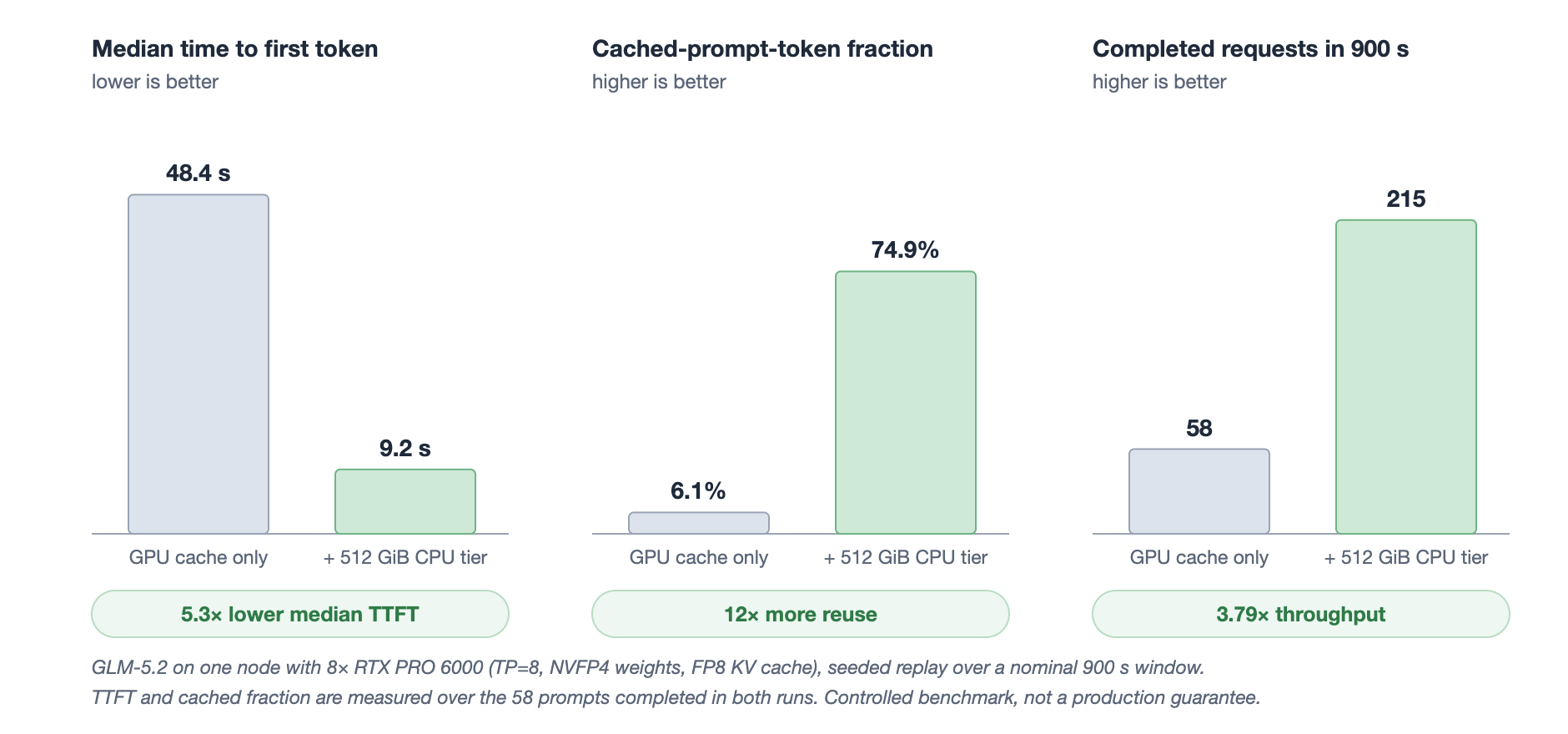Figure 6. Adding a 512 GiB CPU cache tier to GLM-5.2 on one 8x RTX PRO 6000 node raises prefix reuse, which cuts median TTFT and increases completed requests in a controlled replay.

LinkMulti-Model Routing for Cost Optimization 

While replica routing optimizes hardware efficiency, multi-model routing optimizes overall spend. It dictates how much traffic pays frontier API premiums versus running on self-hosted infrastructure. Combining both gives you full control over performance and cost.

Three common policies are:

1. Route by task complexity. Send routine edits, searches, and known Agent Skills to a smaller open model; reserve a frontier model for difficult reasoning or critical changes.

2. Fall back when self-hosted LLM service capacity is constrained. If GPUs cannot scale quickly enough for a burst, use an approved hosted model instead of allowing the queue to grow without bound.

3. Fall back to open models when hosted quotas are exhausted. Keep work moving when a subscription or API reaches a limit.

A CPU-only LiteLLM gateway can implement model selection in front of separate Ray Serve LLM services and external providers. The repository includes a deployable gateway with primary, fallback, and complexity-router configuration, plus a routing-policy guide. LiteLLM's auto-routing documentation covers the underlying complexity of the router. Keyword and skill-aware rules are fast and explainable; a classifier can support richer policies. Explicit user overrides remain important because no router perfectly predicts task difficulty.

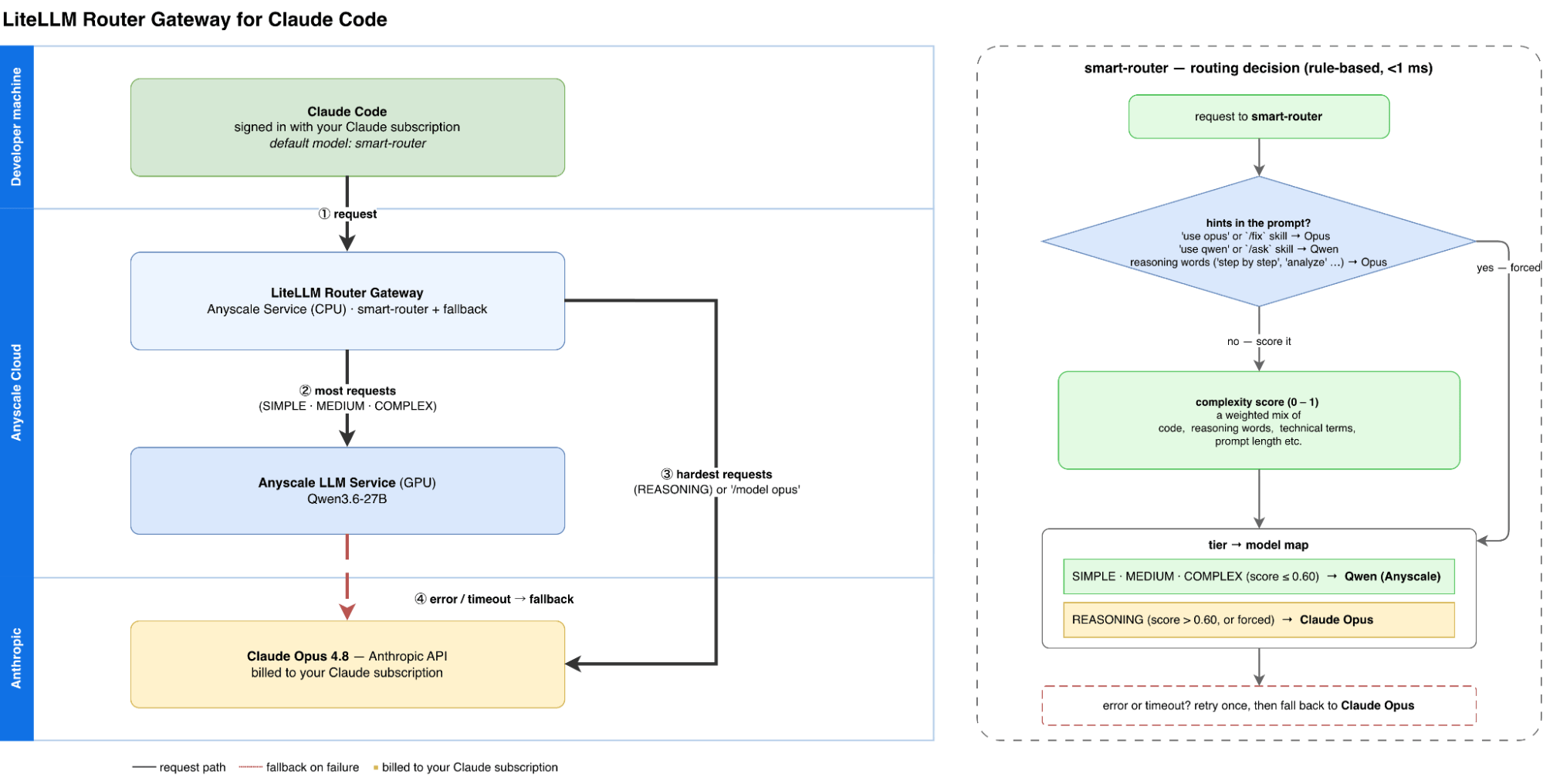Figure 7. LiteLLM Router Gateway: Cost-Aware Model Routing for Claude Code.

In our internal setup, the gateway routes simple requests to Qwen, intermediate to advanced text tasks to GLM, and complex reasoning or multimodal workloads to Claude. To prevent subsequent tool-result steps from unexpectedly changing models mid-stream, the router enforces session stickiness throughout the remaining agent session.

Maintaining this session stickiness is critical for smooth operations. Because coding-agent iterations frequently pass tool outputs without a new user prompt, evaluating routing on a per-request basis risks shifting a single session across disparate models with conflicting chat formats, context bounds, and tool mechanics.

LinkContinuous improvement via observability and post-training

Track system performance across task, model, and platform dimensions using Anyscale service monitoring alongside the Ray Serve LLM dashboard.

High-quality execution traces drive an iterative post-training pipeline. Log multi-turn interactions through an observability platform such as Langfuse, curate and preprocess datasets with Ray Data, detect performance regressions using automated evaluation suites, and post-train open models with SkyRL, a reinforcement learning framework that runs on Ray and Anyscale. Coinbase took this approach for its Onramp fraud agent. It post-trained Qwen3.5-9B with SkyRL on its proprietary fraud data, and the resulting model outperformed Claude Opus 4.5 on all four fraud-detection metrics while cutting end-to-end serving latency by 55%. Each round of post-training feeds the improved model back into production, which turns a static deployment into a self-improving agent flywheel.

/anyscale-workload-llm-serving Follow the guide in https://github.com/anyscale/llm-serving-for-coding-agents/tree/main/part3-optimize and deploy the coding-agent LLM service as written. Validate the generated artifacts in an Anyscale Workspace, deploy them as an Anyscale Service, and test the endpoint with /anyscale-platform-run skill.

LinkOptimize an existing LLM service

Point the serving skill at your current service and the repository's measured optimization example:

/anyscale-workload-llm-serving Deploy an optimized LLM service by following the guidance in https://github.com/anyscale/llm-serving-for-coding-agents/tree/main/part3-optimize. Use this code as a template, inspect my existing service, and adapt the model, GPU, context length, parsers, and performance settings as needed. Benchmark the baseline and optimized configurations with /anyscale-platform-run skill.

Feel free to substitute another LLM; the skill should revalidate model-specific parsers, runtime compatibility, memory fit, and performance settings rather than copying the Qwen configuration unchanged.