Three ways to speed up XGBoost model training

Extreme gradient boosting, or XGBoost, is an efficient open-source implementation of the gradient boosting algorithm. This method is popular for classification and regression problems using tabular datasets because of its execution speed and model performance. But the XGBoost training process can be time consuming.

In a previous blog post, we covered the advantages and disadvantages of several approaches for speeding up XGBoost model training. Check out that post for a high-level overview of each approach. In this article, we’ll dive into three different approaches for reducing the training time of an XGBoost classifier, with code snippets so you can follow along:

• Tree method (gpu_hist)

• Cloud training

• Distributed XGBoost on Ray

Before we jump in, let’s create an XGBoost model using the scikit-learn library to import the make-classification function. This allows you to create a synthetic dataset. Then, we’ll define an XGBoost classifier to train on that dataset.

1
2
3
4
5
6
7
8
9
10
11
12
13
14
15
16
17
from sklearn.datasets import make_classification
from sklearn.model_selection import train_test_split
from xgboost import XGBClassifier
# define dataset
X, y = make_classification(
    n_samples=100000,
    n_features=1000,
    n_informative=50,
    n_redundant=0,
    random_state=1)
# summarize the dataset
print(X.shape, y.shape)
X_train, X_test, y_train, y_test = train_test_split(
    X, y, test_size=0.50, random_state=1)

# define the model
model = XGBClassifier()

This creates an XGBoost classifier that is ready to be trained. Now, let's see how we can train it using the tree method.

LinkTree method

The tree method parameter sets the algorithm used by XGBoost to build boosted trees, as shown in the figure below. By default, an approx algorithm is used, which doesn’t offer the best performance. Switching to the hist algorithm improves performance. However, because both of those algorithms only use the central processing unit (CPU), neither offers outstanding performance overall. 

By enabling the gpu_hist algorithm, as shown in the code sample below, you can train your XGBoost using the graphics processing unit (GPU). This is because running models on the GPU can save a great deal of time compared to running them on the CPU.

Note that when training XGBoost, you can set the depth to which the tree may grow. In the following diagram, the left tree has a depth of 2 and the right tree has a depth of 3. By default, the maximum depth is 6. Bigger trees can better model complex interactions between features, but if they are too deep, they may cause overfitting. Bigger trees also take longer to train. There are also multiple other hyperparameters that control the training process. Finding the best set of hyperparameters for your problem should be automated with a tool like HyperOpt, Optuna, or Ray Tune.

1
2
3
4
5
6
7
8
9
10
11
12
13
14
15
16
17
18
19
20
21
# define the datasets to evaluate each iteration
evalset = [(X_train, y_train), (X_test, y_test)]
#################
model = XGBClassifier(
    learning_rate=0.02,
    n_estimators=10,
    objective="binary:logistic",
    nthread=3,
    tree_method="gpu_hist"  # this enables GPU.
)

import time
print('Lets GO!')
start = time.ctime()
# fit the model
model.fit(X_train, y_train, eval_metric='logloss', eval_set=evalset)

end = time.ctime()
print('all done!')
print('started', start)
print('finished', end)

The tree method learning curve of the XGBoost uses GPU. See the training time with CPU and GPU:

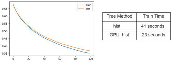
You’ll notice in the figure above that when XGBoost is trained on a large dataset with gpu_hist enabled, training speeds up dramatically with a decrease from 41 seconds (hist) to 23 seconds (gpu_hist). 

LinkThe cloud

Tweaking the tree method is ideal for using our local GPUs to train XGBoost models, but other ways can be more effective. The solution hides in the cloud. Cloud computing allows us to access much more powerful GPUs and in greater numbers than we have available locally. However, this comes at a cost. 

These cloud GPU providers aren’t free, but there are options for training on powerful GPUs, such as the pay-as-you-go solution. This gives you the right to shut down training instances when you finish training, meaning you only pay when you’re using them. 

The XGBoost model used in this article is trained using AWS EC2 instances and checks out the training time results. The process is quite simple. Below is an overview of the steps used to train your XGBoost on AWS EC2 instances:

• Set up an AWS account (if needed)

• Launch an AWS Instance

• Log in and run the code

• Train an XGBoost model

• Close the AWS Instance

To make it simpler, after signing in, choose an Amazon Machine Image (AMI) to launch your virtual machine with EC2, on which you can run XGBoost.

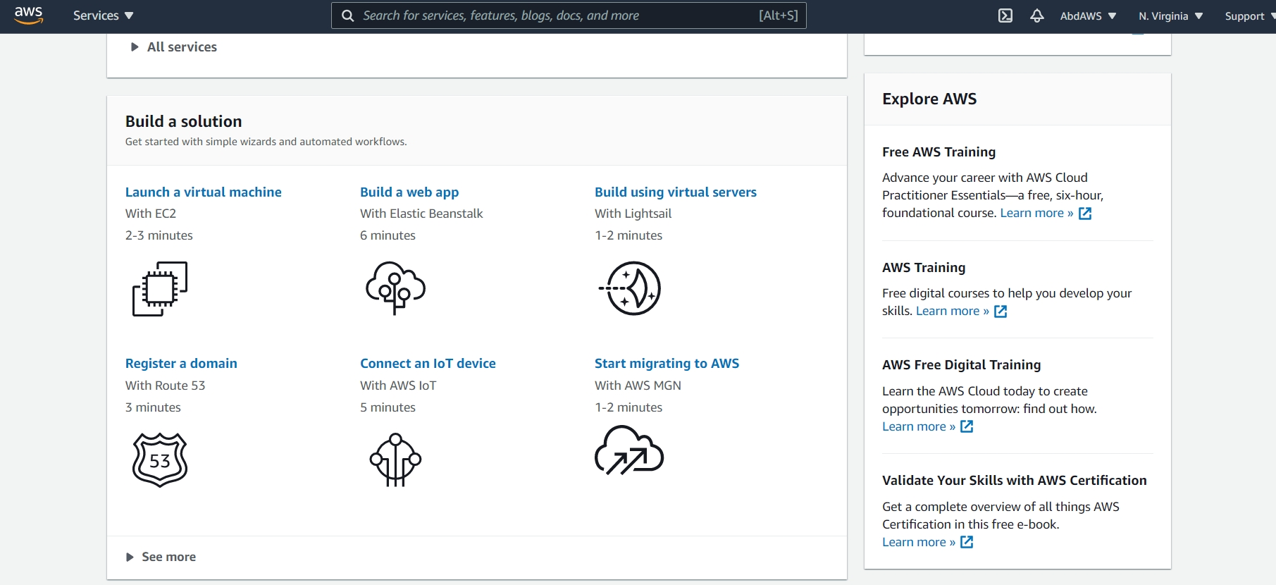
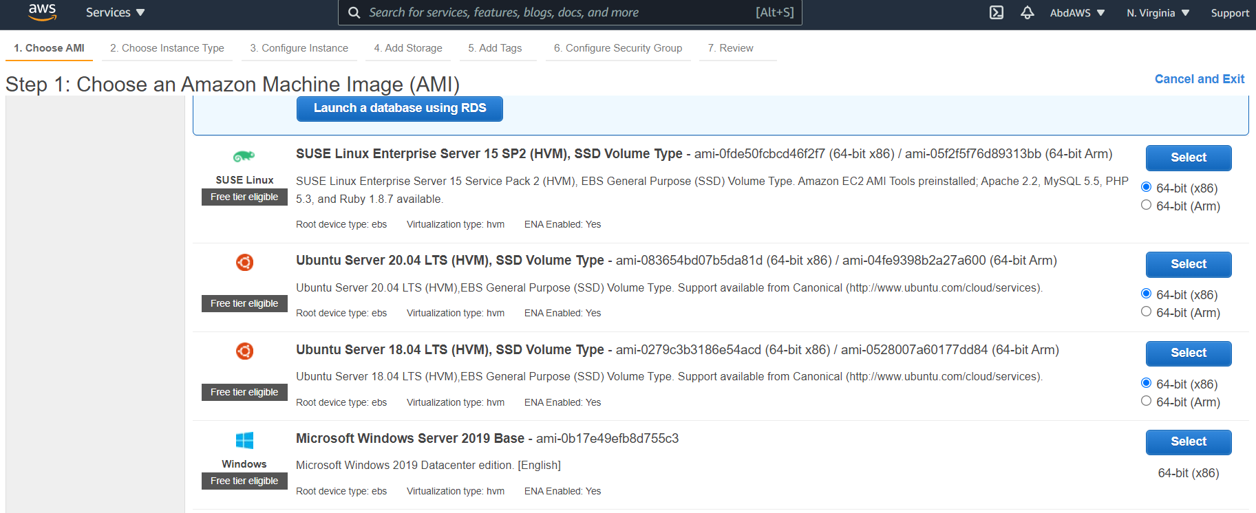
To learn more about how to start an EC2 instance, check out How to Train XGBoost Models in the Cloud with Amazon Web Services. 

Once you launch your instance, you can run the same code you created previously and train XGBoost, with the tree_method set to gpu_hist. Once trained, you’ll notice that training with AWS EC2 is faster compared to using our local GPUs.

LinkDistributed XGBoost training with Ray

So far, you’ve seen that it’s possible to speed up the training of XGBoost on a large dataset by either using a GPU-enabled tree method or a cloud-hosted solution like AWS or Google Cloud. In addition to these two options, there’s a third — and better — solution: distributed XGBoost on Ray, or XGBoost-Ray for short.  

XGBoost-Ray is a distributed learning Python library for XGBoost, built on a distributed computing framework called Ray. XGBoost-Ray allows the effortless distribution of training in a cluster with hundreds of nodes. It also provides various advanced features, such as fault tolerance, elastic training, and integration with Ray Tune for hyperparameter optimization.

The default implementation of XGBoost can only use one GPU and CPU on a single machine. In order to leverage more resources, it’s necessary to use a distributed training method like XGBoost-Ray. Furthermore, if you are working with datasets that are too big to fit in memory of a single machine, distributed training is necessary.

Here’s a diagram of XGBoost-Ray distributed learning with multi-nodes and multi-GPUs:

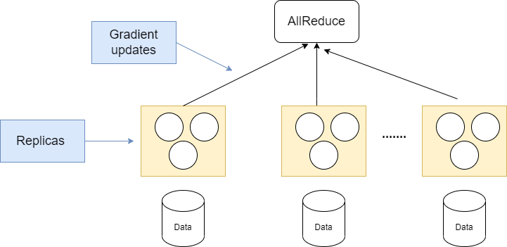
For training, XGBoost-Ray creates training actors for the whole cluster. Then, each of these actors trains on a separate piece of the data. This is called data-parallel training. Actors communicate their gradients using tree-based AllReduce as shown in the figure below.

Here’s what happens to the training time when you train XGBoost with Ray. First, start by getting the XGBoost code that you used before and import the XGBoost-Ray dependencies, such as train and RayParams.

1
2
3
4
5
6
7
8
9
10
11
12
13
14
15
from sklearn.datasets import make_classification
from sklearn.model_selection import train_test_split
# define dataset
X, y = make_classification(
    n_samples=100000,
    n_features=1000,
    n_informative=50,
    n_redundant=0,
    random_state=1)
# summarize the dataset
print(X.shape, y.shape)
X_train, X_test, y_train, y_test = train_test_split(
    X, y, test_size=0.50, random_state=1)

from xgboost_ray import RayDMatrix, RayParams, train

Now that the classifier is ready, you can start configuring your distributed training framework to perform multi-GPU training — in other words, selecting how many actors you should use and the distribution of CPUs and GPUs amongst the actors. You do this with the RayParams object, which you use to divide CPUs and GPU among actors. Here, you train the XGBoost on a machine with six CPUs and two GPUs. For multi-CPU and GPU training, select the number of actors to be at least two with three CPUs and one GPU each. The actors will be automatically scheduled by Ray on your cluster.

Because we are only using one machine in our example, both of those actors will be put on it, but we would be able to use the same code with a cluster of dozens or hundreds of machines. Note that the data is passed to XGBoost-Ray using a RayDMatrix object. This object stores data in a sharded way so that each actor can access its part of the data to perform training.

1
2
3
4
5
6
7
8
9
10
11
12
13
14
15
16
17
18
19
20
21
22
23
train_set = RayDMatrix(X_train, y_train)
eval_set = RayDMatrix(X_test, y_test)
evals_result = {}
bst = train(
    {
        "objective": "binary:logistic",
        "eval_metric": ["logloss", "error"],
    },
    train_set,
    num_boost_round=10,
    evals_result=evals_result,
    evals=[(train_set, "train"), (eval_set, "eval")],
    verbose_eval=True,
    ray_params=RayParams(
        num_actors=2,
        gpus_per_actor=1,
        cpus_per_actor=3,  # Divide evenly across actors per machine
    ))
bst.save_model("model.xgb")
print("Final training error: {:.4f}".format(
    evals_result["train"]["error"][-1]))
print("Final validation error: {:.4f}".format(
    evals_result["eval"]["error"][-1]))

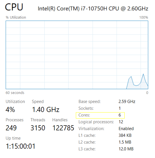
The machine used for running the XGBoost training in this example has six cores:

LinkComparing results 

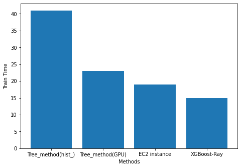
Finally, it’s time to compare the results to see which method speeds up the training of XGBoost the most. As you can see in the table below, distributed training with Ray was the most effective method for reducing the training time, thanks to the use of features like multi-CPU training, multi-GPU training, fault tolerance, and support for configurable parameters like the RayParam function. XGBoost-Ray could be used to reduce the training time even further by using a cluster of machines instead of one as in our example.

LinkConclusion

In this article, we explored several methods that you can use to speed up the training of the XGBoost classifier. Ultimately, we found that XGBoost distributed training with Ray beats all other techniques in terms of training speed. This is because XGBoost-Ray includes multi-node training, full CPU support, full GPU support, and configurable parameters like RayParam.

In the next article in this series, we’ll explore how to use Ray Serve to deploy XGBoost models. Or, if you’re interested in learning more about Ray and XGBoost, check out the additional resources below:

• Register for our upcoming webinar on how to simplify and scale your XGBoost model using Ray on Anyscale

• Read how the Ray team at Ant Group used XGBoost on Ray and other Ray machine learning libraries to implement an end-to-end AI pipeline in one job

• Explore the XGBoost-Ray documentation